14 Dynamic Branch Prediction

 

The objectives of this module are to discuss how control hazards are handled in the MIPS architecture and to look at more realistic branch predictors.

 

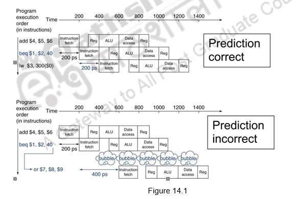
In the previous module, we discussed about the basics of control hazards and discussed about how the compiler handles control hazards. We have seen that longer pipelines can’t readily determine the branch outcome early and the stall penalty becomes unacceptable in such cases. As far as the MIPS pipeline is concerned, we can predict branches as not taken and fetch instructions after the branch, with no delay. Figure 14.1 shows the predict not taken approach, when the prediction is correct and when the prediction is wrong. When the prediction is right, that is, when the branch is not taken, there is no penalty to be paid. On the other hand, when the prediction is wrong, one bubble is created and the next instruction is fetched from the target address. Here, we assume that the branch is resolved in the IF stage itself.

 

Let us consider the following sequence of operations.

36	sub	$10, $4, $8
40	beq	$1, $3, 7 # PC-relative branch to 40 + 4 + 7 * 4 = 72
44	and	$12, $2, $5
48	or	$13, $2, $6

52	add	$14, $4, $2
56	slt	$15, $6, $7
. . .
72	lw	$4, 50($7)

 

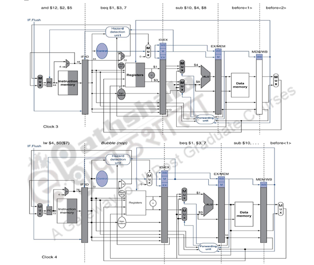
Figure 14.2 shows what happens in the MIPS pipeline when the branch is taken. The ID stage of clock cycle 3 determines that a branch must be taken, so it selects the target address as the next PC address (address 72) and zeros the instruction fetched for the next clock cycle. Clock cycle 4 shows the instruction at location 72 being fetched and the single bubble or nop instruction in the pipeline as a result of the taken branch. The associated data hazards that might arise in the pipeline when the branch is resolved in the second stage has already been discussed in the earlier modules.

 

Now, we shall discuss the second type of branch prediction, viz. dynamic branch prediction. Branch Prediction is the ability to make an educated guess about which way a branch will go – will the branch be taken or not. In the case of dynamic branch prediction, the hardware measures the actual branch behavior by recording the recent history of each branch, assumes that the future behavior will continue the same way and make predictions. If the prediction goes wrong, the pipeline will stall while re-fetching, and the hardware also updates the history accordingly. The comparison between the static prediction discussed in the earlier module and dynamic prediction is given below:

 

•  Static

–  Techniques

• Delayed Branch

• Static prediction

–  No info on real-time behavior of programs

–  Easier/sufficient for single-issue

–  Need h/w support for better prediction

• Dynamic

–  Techniques

• History-based Prediction

–  Uses info on real-time behavior

–  More important for multiple-issue

–  Improved accuracy of prediction

 

In the case of dynamic branch prediction, the hardware can look for clues based on the instructions, or it can use past history. It maintains a History Table that contains information about what a branch did the last time (or last few times) it was executed. The performance of this predictor is

 

Performance = ƒ(accuracy, cost of mis-prediction)

 

There are different types of dynamic branch predictors. We shall discuss each of them in detail. The seven schemes that we shall discuss are as follows:

 

1. 1-bit Branch-Prediction Buffer

2. 2-bit Branch-Prediction Buffer

3. Correlating Branch Prediction Buffer

4. Tournament Branch Predictor

5. Branch Target Buffer

6. Return Address Predictors

7.  Integrated Instruction Fetch Units

 

1-bit Branch-Prediction Buffer: In this case, the Branch History Table (BHT) or Branch Prediction Buffer stores 1-bit values to indicate whether the branch is predicted to be taken / not taken. The lower bits of the PC address index this table of 1-bit values and get the prediction. This says whether the branch was recently taken or not. Based on this, the processor fetches the next instruction from the target address / sequential address. If the prediction is wrong, flush the pipeline and also flip prediction. So, every time a wrong prediction is made, the prediction bit is flipped. Usage of only some of the address bits may give us prediction about a wrong branch. But, the best option is to use only some of the least significant bits of the PC address.

 

The prediction accuracy of a single bit predictor is not very high. Consider an example of a loop branch taken nine times in a row, and then not taken once. Even in simple iterative loops like this, the 1-bit BHT will cause 2 mispredictions (first and last loop iterations): first time through the loop, when it predicts exit instead of looping, and the end of the loop case, when it exits instead of looping as before. Therefore, the prediction accuracy for this branch that has taken 90% of the time is only 80% (2 incorrect predictions and 8 correct ones). So, we have to look at predictors with higher accuracy.

 

2-bit predictor: This predictor changes prediction only on two successive mispredictions. Two bits are maintained in the prediction buffer and there are four different states. Two states corresponding to a taken state and two corresponding to not taken state. The state diagram of such a predictor is given below.

 

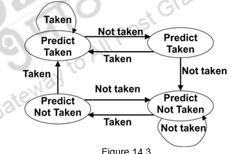
Figure 14.3

 

Advantage of this approach is that a few atypical branches will not influence the prediction (a better measure of ―the common case‖). Only when we have two successive mispredictions, we will switch prediction. This is especially useful when multiple branches share the same counter (some bits of the branch PC are used to index into the branch predictor). This can be easily extended to N-bits. Suppose we have three bits, then there are 8 possible states and only when there are three successive mispredictions, the prediction will be changed. However, studies have shown that a 2-bit predictor itself is accurate enough.

 

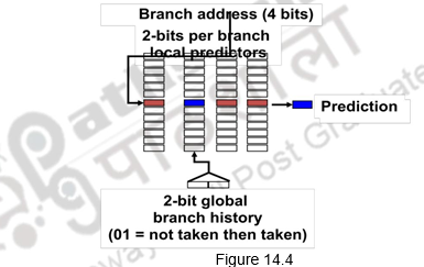
Correlating branch predictors: The 2-bit predictor schemes use only the recent behavior of a single branch to predict the future behavior of that branch. But, many a times, we find that the behavior of one branch is dependent on the behavior of other branches. There is a correlation between different branches. Branch Predictors that use the behavior of other branches to make a prediction are called Correlating or two-level predictors. They make use of global information rather than local behavior information. The information about any number of earlier branches can be maintained. For example, if we maintain the information about three earlier branches, B1, B2 and B3, the behavior of the current branch now depends on how these three earlier branches behaved. There are eight different possibilities, from all three of them not taken (000) to all of them taken (111). There are eight different predictors maintained and each one of them will be maintained as a 1-bit or 2-bit predictor as discussed above. One of these predictors will be chosen based on the behavior of the earlier branches and its prediction used. In general, it is an (m,n) predictor, with global information about m branches and each of the predictors maintained as an n-bit predictor. Figure 14.4 shows an example of a correlating predictor, where m=2.

 

 

Tournament predictors: The next type of predictor is a tournament predictor. This uses the concept of ―Predicting the predictor‖ and hopes to select the right predictor for the right branch. There are two different predictors maintained, one based on global information and one based on local information, and the option of the predictor is based on a selection strategy. For example, the local predictor can be used and every time it commits a mistake, the prediction can be changed to the global predictor. Otherwise, the switch can be made only when there are two successive mispredictions. Such predictors are very popular and since 2006, tournament predictors using » 30K bits are used in processors like the Power5 and Pentium 4. They are able to achieve better accuracy at medium sizes (8K – 32K bits) and also make use of very large number of prediction bits very effectively. They are the most popular form of multilevel branch predictors which use several levels of branch-prediction tables together with an algorithm for choosing among the multiple predictors.

 

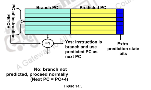
Branch Target Buffer (BTB): With all the branch prediction schemes discussed earlier, we still need to calculate the target address. This gives 1-cycle penalty for a taken branch. If we need to reduce the branch penalty further, we need to fetch an instruction from the destination of a branch quickly. You need the next address at the same time as you’ve made the prediction. This can be tough if you don’t know where that instruction is until the branch has been figured out. The solution is a table that remembers the resulting destination addresses of previous branches. This table is called the Branch Target Buffer (BTB) that caches the target addresses and is indexed by the complete PC value when the instruction is fetched. That is, even before we have decoded the instruction and identified that it is a branch, we index into the BTB. When the PC is used to fetch the next instruction, it is also used to index into the BTB. The BTB stores the PC value and the corresponding target addresses for some of the most recent taken branches. If there is a hit and the instruction is a branch predicted taken, we can fetch the target immediately. This gives a zero cycle penalty for conditional branches. If there is no entry in the BTB, we follow the usual procedure and if it is a taken branch, make an entry in the BTB. On the other hand, if the prediction is wrong, the penalty has to be paid and the BTB entry will have to be removed. This is illustrated in Figure 14.5.

 

Let us discuss an example problem to illustrate the concepts studied. Consider the table given below.

 

Determine the total branch penalty for a BTB using the above data. Assume

• Prediction accuracy of 90%

• Hit rate in the buffer of 90% & 60% of the branches are taken

 

Branch Penalty = Percent buffer hit rate X Percent incorrect predictions X 2 + ( 1 – percent buffer hit rate) X

Taken branches X 2

 

Branch Penalty = ( 90% X 10% X 2)  + (10% X 60% X 2)

 

Branch Penalty = 0.18 + 0.12    = 0.30 clock cycles

 

Return Address Predictors: Next we shall at look at the challenge of predicting indirect jumps, that is, jumps whose destination address varies at run time. It is very hard to predict the address for indirect jumps (indirect procedure calls, returns, case statements). If we look at the SPEC89, 85% of such branches are from procedure returns. Though procedure returns can be predicted with a branch-target buffer, the accuracy of such a prediction technique can be low if the procedure is called from multiple sites and the calls from one site are not clustered in time. For example, in SPEC CPU95, an aggressive branch predictor achieves an accuracy of less than 60% for such return branches. To overcome this problem, some designs use a small buffer of return addresses operating as a stack. This structure caches the most recent return addresses: pushing a return address on the stack at a call and popping one off at a return. If the cache is sufficiently large (i.e., as large as the maximum call depth), it will predict the returns perfectly.

 

Integrated Instruction Fetch Unit: To meet the demands of modern processors that issue multiple instructions every clock cycle, many recent designers have chosen to implement an integrated instruction fetch unit, as a separate autonomous unit that feeds instructions to the rest of the pipeline. An integrated instruction fetch unit integrates several functions:

 

1. Integrated branch prediction—The branch predictor becomes part of the instruction fetch unit and is constantly predicting branches, so as to drive the fetch pipeline.

 

2. Instruction prefetch—To deliver multiple instructions per clock, the instruction fetch unit will likely need to fetch ahead. The unit autonomously manages the prefetching of instructions, integrating it with branch prediction.

 

3. Instruction memory access and buffering—When fetching multiple instructions per cycle a variety of complexities are encountered, including the difficulty that fetching multiple instructions may require accessing multiple cache lines. The instruction fetch unit encapsulates this complexity, using prefetch to try to hide the cost of crossing cache blocks. The instruction fetch unit also provides buffering, essentially acting as an on-demand unit to provide instructions to the issue stage as needed and in the quantity needed.

 

Thus, as designers try to increase the number of instructions executed per clock, instruction fetch will become an ever more significant bottleneck, and clever new ideas will be needed to deliver instructions at the necessary rate.

 

To summarize, we have pointed out in this module that prediction is important to handle branch hazards and dynamic branch prediction is more effective. We have discussed different types of predictors. A 1-bit predictor uses one bit prediction, but is not very accurate. A 2-bit predictor has improved prediction accuracies and changes prediction only when there are two successful mispredictions. Correlating branch predictors correlate recently executed branches with the next branch. Tournament Predictors use more resources to competitive solutions and pick between these solutions. A Branch Target Buffer includes the branch address and prediction. Return address stack is used for prediction of indirect jumps. Finally, an integrated instruction fetch unit treats the instruction fetch as a single complicated process and tries to look at different techniques to ensure that a steady stream of instructions are fed to the processor.