Near Optimal Coflow Scheduling in Networks
Mosharaf Chowdhury*, Samir Khuller\({}^{\dagger}\), Manish Purohit\({}^{\ddagger}\), Sheng Yang**, Jie You*
*: University of Michigan, \({}^{\dagger}\): Northwestern University, \({}^{\ddagger}\): Google Research, **: University of Maryland, College ParkIntroduction
Global data center traffic by destination in 2021
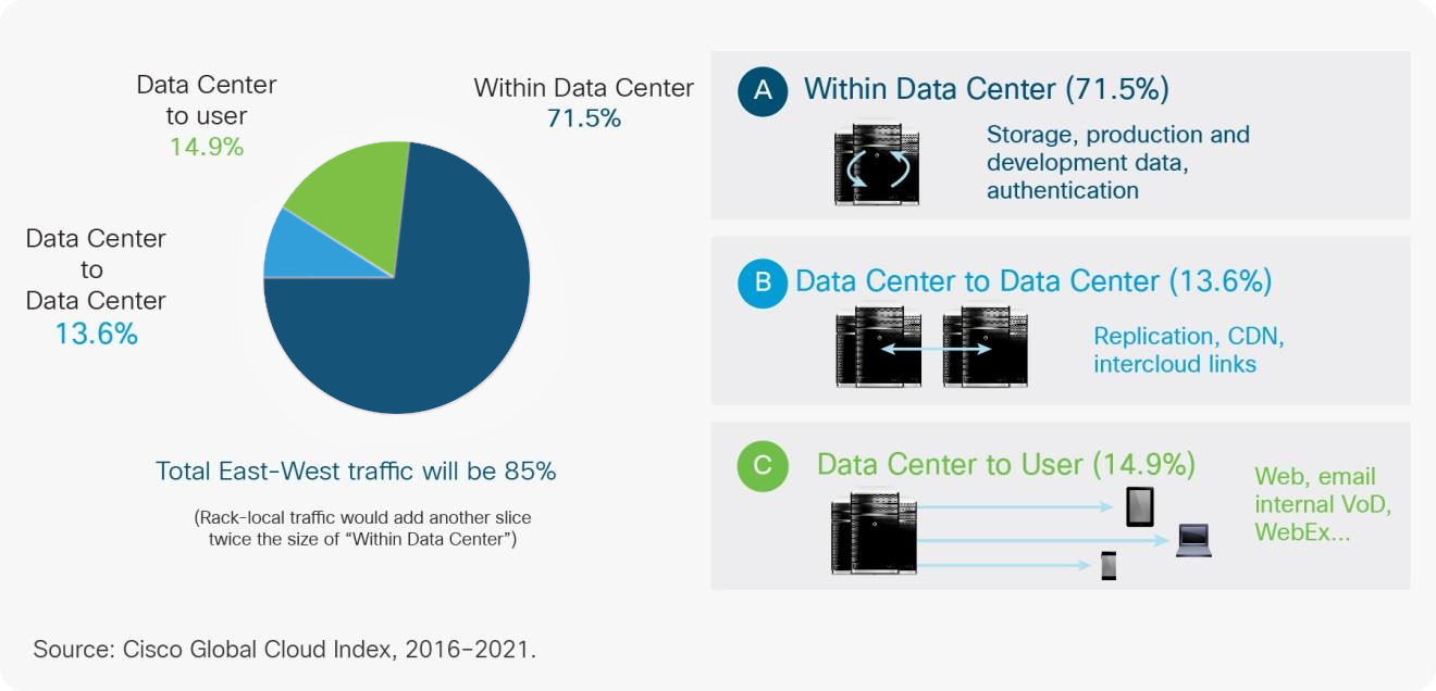
From Cisco Global Cloud Index: Forecast and Methodology, 2016–2021 White Paper: https://www.cisco.com/c/en/us/solutions/collateral/service-provider/global-cloud-index-gci/white-paper-c11-738085.pdf
Coflow Scheduling*
- Optimize data transmission for jobs within a data center.
- Machines can communicate with each other directly
- Uniform machine/capacity.
*: first modeled by Chowdhury and Stoica in Coflow: A networking abstraction for cluster applications, HotNets 2012
Example of a Coflow
Coflow in Matrix Form
Problem Description
- \(n\) coflows, each represented as matrix \(D^j = [d^j_{io}]\).
- \(d^j_{io}\): demand of job \(j\) from input port \(i\) to output port \(o\).
- For every coflow \(j\):
- \(r_j\): release time
- \(w_j\): weight
- Minimize: \(\sum_{i=1}^n w_j\cdot C_j\).
- \(C_j\): completion time. A coflow is finished when all its flows are finished.
- Discrete time.
- At each time slot an input/output port can send/receive at most one unit of flow.
How to Schedule a Single Coflow?
Schedule a Single coflow
Schedule a Single coflow
Schedule a Single coflow
Schedule a Single coflow
Concurrent Open Shop
- \(n\) jobs to be scheduled on \(m\) different machines.
- Each job \(j\) consists of \(m\) tasks for each machine. For machine \(i\), there is an task that takes \(d^j_i\) time to finish.
- Different tasks of the same job can take place at the same time.
- A job is finished when all its tasks are finished.
- Minimize weighted completion time.
Relation to Coflow Scheduling
Hardness for Concurrent Open Shop
- NP-hard* (UGC-hard**) to get \((2 - \epsilon)\) approximation for any \(\epsilon > 0\).
- Implies same lower bound for coflow scheduling.
*: Sushant Sachdeva, Rishi Saket, Optimal inapproximability for scheduling problems via structural hardness for hypergraph vertex cover, CCC 2013
**: Nikhil Bansal, Subhash Khot, Inapproximability of hypergraph vertex cover and applications to scheduling problems, ICALP 2010
A Brief History
A Brief History
- Chowdhury and Stoica* first model the coflow scheduling problem.
- Chowdhury, Zhong, and Stoica\({}^{\dagger}\) give effective heuristic to optimize coflow completion time.
*: Mosharaf Chowdhury, Ion Stoica, Coflow: A networking abstraction for cluster applications, HotNets 2012
\(\dagger\): Mosharaf Chowdhury, Yuan Zhong, Ion Stoica, Efficient Coflow Scheduling with Varys, SIGCOMM 2014
A Brief History, Theoretical Side
Qiu, Stein, and Zhong proved the following for coflow scheduling in SPAA 2015:
| Zero release time | Arbitrary release time | |
| Randomized | \(8 + \frac{16\sqrt{2}}{3}\) | \(9 + \frac{16\sqrt{2}}{3}\) |
| Deterministic | \(\frac{64}{3}\) | \(\frac{76}{3}^{*}\) |
Z. Qiu, C. Stein, and Y. Zhong, Minimizing the total weighted completion time of coflows in datacenter networks, SPAA 2015. *:The authors claimed a ratio of \(\frac{67}{3}\), but the proof only holds when all release times are the same.
A Brief History, Theoretical Side
In SPAA 2016, Khuller and Purohit* improve upon this via a black box reduction to Concurrent Open Shop Problem and get
- Zero release time (deterministic): 8-approx
- Arbitrary release time (deterministic): 12-approx
*: S. Khuller and M. Purohit, Brief Announcement: Improved Approximation Algorithms for Scheduling Co-Flows, SPAA 2016
A Brief History, Current Best Results
- Zero release time*, \({}^{\dagger}\): 4-approx
- Arbitrary release time*, \({}^{\dagger}\): 5-approx
- Combinatorial using primal-dual*
- : joint work with Saba Ahmadi, Samir Khuller, and Manish Purohit, On Scheduling Coflows, IPCO 2017.
\(\dagger\) : an independent work: A New Improved Bound for Coflow Scheduling by Mehrnoosh Shafiee, Javad Ghaderi in SPAA 2017, give the same bound but used a different LP.
A Brief History, Implementations
In SIGCOMM 2018, Agarwal et al. implemented Sincronia which uses a similar primal-dual algorithm without release time. Evaluation results suggest that it not only admits a practical, near-optimal design but also improves upon state-of-the-art network designs for coflows.
Saksham Agarwal, Shijin Rajakrishnan, Akshay Narayan, Rachit Agarwal, David Shmoys, Amin Vahdat, Sincronia: near-optimal network design for coflows, SIGCOMM 2018.
Coflow Scheduling in Networks
- Optimize data transmission for jobs across data centers.
- Data centers may be directly connected, or connected via multiple routers.
- Network modeled as an directed graph with non-uniform structure.
- Sharing a link within a coflow or between coflows is allowed.
- Spliting and merging a flow is also allowed.
Example of a Coflow in Networks
Problem Description
- A weighted directed graph \(G = (V, E)\) representing the network.
- Weight of an edge is its capacity.
- \(n\) coflows, each represented as a matrix \(D^j = [d^j_{io}]\).
- \(d^j_{io}\): demand of job \(j\) from node \(i\) to node \(o\).
- Either a path is given, or there is no limitation on paths.
- For every coflow \(j\):
- \(r_j\): release time
- \(w_j\): weight
- Minimize: \(\sum_{i=1}^n w_j\cdot C_j\).
- \(C_j\): completion time. A coflow is finished when all its flows are finished.
- Discrete time.
- An edge can be shared within a coflow or between coflows, as long as the total bandwidth is within its capacity.
Problem Description, Continued
- A schedule would decide at each time slot:
- Which flows to send.
- How shall we route each flow.
- At what rate.
- Solution can be fractional.
- Naturally required by data transmission.
- Different from the switch based coflow scheduling problem, where the main difficulty is finding an integral solution.
- The main difficulty comes from coordinating multiple coflows.
Single Path Model and Free Path Model
- Single path model:
- Path for each flow \(f^i_j\) given as \(p^i_j\).
- Only need to decide the rate for each flow at each time.
- Edge bandwidths need to be respected.
- Free path model:
- Path for a flow \(f^i_j\) not specified.
- Need to find routes for every flow.
- Data can split and merge at vertices to utilize all possible links and their capacities.
- Edge bandwidths need to be respected.
Existing Results
- Jahanjou, Kantor, and Rajaraman* give a constant approximation (\(17.53\)) algorithm for the single path model.
- In the same paper*, the authors give a tight \(O\left(\frac{\log |E|}{\log \log |E|}\right)\) algorithm for the case where you need to pick a single path for each demand.
- You and Mosharaf\({}^{\dagger}\) introduce the free path model, and give a heuristic for the unweighted case without theoretical bound.
*: Hamidreza Jahanjou, Erez Kantor, Rajmohan Rajaraman, Asymptotically Optimal Approximation Algorithms for Coflow Scheduling, 2017 SPAA \(\dagger\): Jie You, Mosharaf Chowdhury, Terra: Scalable Cross-Layer GDA Optimizations, 2019 in progress
Our Contributions
- A tight \(2\) approximation randomized algorithm for both models when release times and demands are polynomial sized.
- NP-hard to get \((2-\epsilon)\) approximation for any \(\epsilon > 0\).
- A \((2 + \epsilon)\) randomized approximation algorithm when release times and demands are super-polynomial sized.
- Experiments show significant improvements on existing algorithms.
Algorithm
Algorithm Sketch
- Single Coflow:
- Multi commodity flow
- Can be solved optimally in polynomial time.
- Multiple Coflows:
- Time indexed LP
- Stretching to round the solution.
Time Indexed LP
\(x_j^i(t)\) is the fraction of flow \(i\) in job \(j\) that is finished at time \(t\). \(X_j(t)\) is the total fraction of job \(j\) that is finished by time \(t\).
Time Indexed LP, Completion Time
Start with thinking \(x_j(t)\in \{0, 1\}\).
Constraints for Single Path Model
\[\sum_{p_j^i\ni e} x^i_j(t)\cdot \sigma^i_j \leq c(e), \forall e\in E, \forall t\in T\]
Constraints for Free Path Model
- \(x^i_j(t, e)\): the fraction of flow \(f^i_j\) transmitted through edge \(e\) in time slot \(t\).
- \(x^i_j(t)\): the total fraction of flow \(f^i_j\) that is transmitted in time slot \(t\).
Stretching
Stretching
Stretching
Stretching
Stretching
Experiments
Future Directions
- Improve Efficiency
- It takes quite long to solve the linear program.
- Is it possible to avoid solving LP?
- Or limit the LP without sacrificing too much on approximation ratio?
- Shed light on switch model
- Model precedence constraints
Q & A
Powered by
- Reveal.js: the slide framework
- magic.css: some animations
- org-mode and org-reveal: for making the slides