


 where
where  is
either 0 or 1, and is also either 0 or 1. Note that there are
only four possible functions of this sort: the constant functions 0
and
is
either 0 or 1, and is also either 0 or 1. Note that there are
only four possible functions of this sort: the constant functions 0
and  , the identity function
  , and the reverse function. But
we are given the function in the form of a complicated expression, so
that we do not know which of the four functions
, and the reverse function. But
we are given the function in the form of a complicated expression, so
that we do not know which of the four functions  really is. We can
of course simply compute on both inputs and then see which it
is. But that takes two separate computations, hence roughly twice as
long as just one such computation. Suppose however that we do not want
to know which of the four functions is; rather all we want to know
is whetehr is ``balanced'' or not--where balanced means that the
values of are both 0 and , ie is not constant. Again it
seems that to find out, we'd have to compute on both inputs and
see, and that would take two separate computations. What Deutsch
discovered is that, if is represented via a system of qubits, it
is possible to manipulate the system so that all the needed
computations are done in parallel, and so that when a
measurement is finally made at the end, the result will reveal whether
is balanced or not, even though it will not reveal exactly which
function is.
really is. We can
of course simply compute on both inputs and then see which it
is. But that takes two separate computations, hence roughly twice as
long as just one such computation. Suppose however that we do not want
to know which of the four functions is; rather all we want to know
is whetehr is ``balanced'' or not--where balanced means that the
values of are both 0 and , ie is not constant. Again it
seems that to find out, we'd have to compute on both inputs and
see, and that would take two separate computations. What Deutsch
discovered is that, if is represented via a system of qubits, it
is possible to manipulate the system so that all the needed
computations are done in parallel, and so that when a
measurement is finally made at the end, the result will reveal whether
is balanced or not, even though it will not reveal exactly which
function is.
The idea is roughly this: we start with two qubits, A and B, one in
state  and one in state
  ; these represent the two possible
inputs to . We will feed them both to at the same time, in
superposition; that is, we feed the AB system (in state
; these represent the two possible
inputs to . We will feed them both to at the same time, in
superposition; that is, we feed the AB system (in state  to .
But how do we do this? There are several tricks involved, and we will
not be able to give complete details and justifications; but the steps
will be clear enough to follow.
to .
But how do we do this? There are several tricks involved, and we will
not be able to give complete details and justifications; but the steps
will be clear enough to follow.
First, we pass AB through a transformation  called the Hadamard
transformation (gate). This transforms into
called the Hadamard
transformation (gate). This transforms into
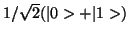 ,
and into
,
and into
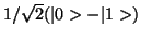 . So transforms AB =
into
. So transforms AB =
into
 So far
has not come into the processing.
So far
has not come into the processing.
Now we pass the above result through the function . But because of
constraints posed by the nature of quantum systems, this has to be
done in a special way. is repesented as a special gate that takes
any state  and produces
 , where the addition is mod 2.
Note that, classically, we would have to do this twice, once for
, where the addition is mod 2.
Note that, classically, we would have to do this twice, once for  and once for
  , to find what does to these two inputs. But
quantum-mechanically, we do both at once, in parallel, with a single
gate applied to the superposition from the earlier step (where AB
was passed through the Hadamard gate ).
, to find what does to these two inputs. But
quantum-mechanically, we do both at once, in parallel, with a single
gate applied to the superposition from the earlier step (where AB
was passed through the Hadamard gate ).
Finally we pass this result once more through the gate . Now it
turns out that by simply looking at (measuring) the A-qubit, we can
tell whether is balanced or not. For in both constant (unbalanced) cases, the
A-qubit has value 0, and in both balanced cases it is 1. (The B-value
turns out to be 1 in all cases, and so holds no useful information
that might reveal exactly which function is.)
Here is the detailed computation for the constant function
 .
.
Step 1: apply Hadamard to to get
 .
We will now suppress the
.
We will now suppress the  and the kets for ease of writing. But
be careful: 0 and 1 will usually mean states, not numbers.
and the kets for ease of writing. But
be careful: 0 and 1 will usually mean states, not numbers.
Step 2: apply the
gate, to get
00 --> 0,0+f(0) = 00

01 --> 0,1+f(0) = 01

10 --> 1,0+f(1) = 10

11 --> 1,1+f(1) = 11
And thus the total result is 00 - 01 + 10 - 11.
has in fact done
nothing at all to the input! But we had to work it out to see; the
other functions are similar, but in those it does do something.
Step 3: apply Hadamard again, to get
(0+1)(0+1) - (0+1)(0-1) + (0-1)(0+1) - (0-1)(0-1)

= (00 + 01 + 10 + 11) - (00 - 01 + 10 - 11) + (00 + 01 - 10 - 11) - (00 - 01 - 10 + 11)

=  00 + 01 + 10 + 11  -  00 + 01 - 10 + 11  +  00 + 01 - 10 - 11  -  00 + 01 + 10 - 11

=  01 + 01 + 01 + 01
which really is just 01, since we suppressed the factors of 1/2, and there were two of those. Thus the final result has an A-qubit value of 0 and a B-qubit value of 1.