Image Filtering Tutorial
CMSC 426: Image Processing [Spring 2016]
TA: Peratham Wiriyathammabhum (MyFirstName-AT-cs.umd.edu)
Contents
Load any image
%# this sample image is from Kullasatree Magazine June 2015.
%# http://iconosquare.com/p/996193116531919677_1512351217
I = imread('sample2.jpg');
I = rgb2gray(I);
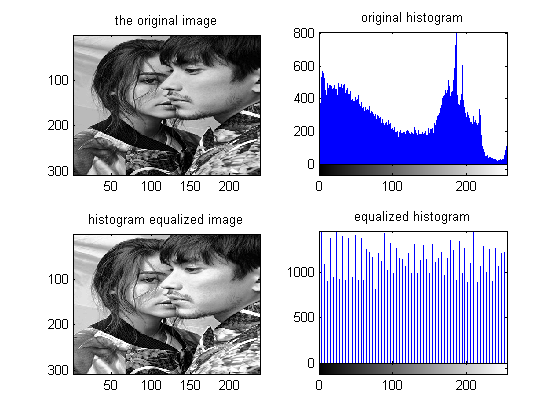
Histogram equalization
%# convert to grayscale images
im = double(I);
%# plot
figure;
subplot(2,2,1);
imagesc(im);
colormap(gray);
title('the original image');

%# histogram plot
subplot(2,2,2);
imhist(I);
title('original histogram');
%# histogram equalization
%# http://www.mathworks.com/help/hdlcoder/examples/image-enhancement-by-histogram-equalization.html
he = histeq(I);

%# plot equalizaed image
subplot(2,2,3);
imagesc(he);
colormap(gray);
title('histogram equalized image');
%# plot new histogram
subplot(2,2,4);
imhist(he);
title('equalized histogram');
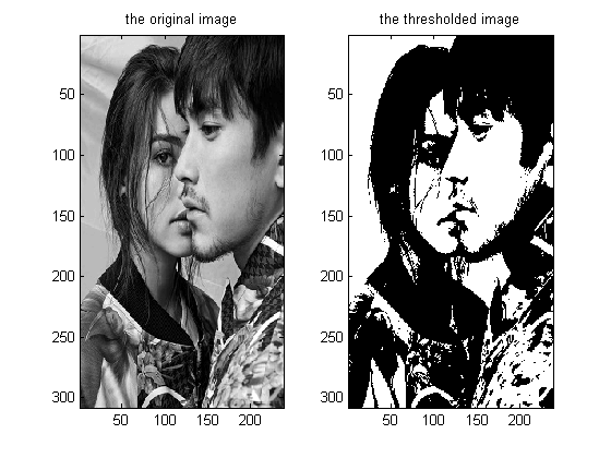
Threshold image
T = 128;
t = im;
t(im <= T) = 0;
t(im > T) = 1;

%# plot
figure;
subplot(1,2,1);
imagesc(im);
colormap(gray);
title('the original image');
subplot(1,2,2);
imagesc(t);
colormap(gray);
title('the thresholded image');
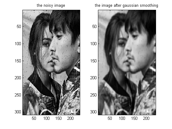
Smooth image
add noise
noise_type = 'salt & pepper'; % 'gaussian' or 'poisson' are also valid
noises = imnoise(im, noise_type, 0.02);
nim = im;
nim(noises == 0) = 0;

% smoothing parameter for gaussian filter
sigma = 1.5;
%# Create the gaussian filter with hsize = [w w] and sigma = sigma
%# where w = sigma * 6  + 1
w = sigma * 6 + 1;
G = fspecial('gaussian',[w w], sigma);
%# Filter it with border replication
o = imfilter(nim, G, 'replicate');

%# plot
figure;
subplot(1,2,1);
imagesc(nim);
colormap(gray);
title('the noisy image');
subplot(1,2,2);
imagesc(o);
colormap(gray);
title('the image after gaussian smoothing');
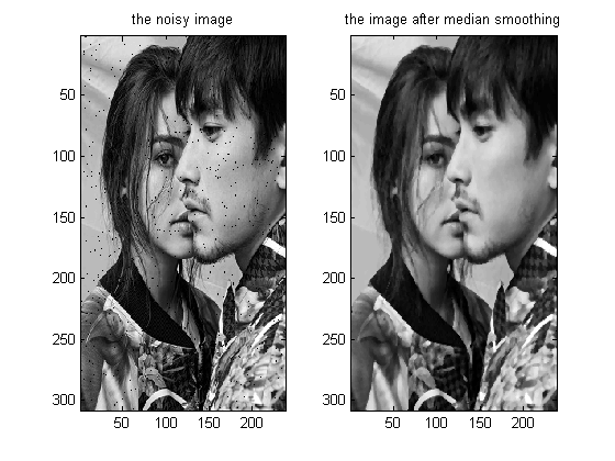
Median smoothing
add noise
noise_type = 'salt & pepper'; % 'gaussian' or 'poisson' are also valid
noises = imnoise(im, noise_type, 0.02);
nim = im;
nim(noises == 0) = 0;

% smoothing parameter for gaussian filter
m = medfilt2(nim, [3 3]);

%# plot
figure;
subplot(1,2,1);
imagesc(nim);
colormap(gray);
title('the noisy image');
subplot(1,2,2);
imagesc(m);
colormap(gray);
title('the image after median smoothing');
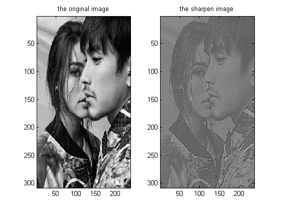
Sharpen image
%# for filters check out topics 17,4,5
G = [0 -1 0; -1 5 -1;0 -1 0];

%# Filter it with border replication
s = imfilter(im, G, 'replicate');

%# plot
figure;
subplot(1,2,1);
imagesc(im);
colormap(gray);
title('the original image');
subplot(1,2,2);
imagesc(s);
colormap(gray);
title('the sharpen image');
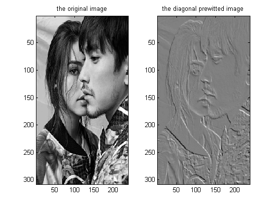
Diagonal prewitt on image
P = [0 1 1; -1 0 1;-1 -1 0];

%# Filter it with border replication
dp = imfilter(im, P, 'replicate');

%# plot
figure;
subplot(1,2,1);
imagesc(im);
colormap(gray);
title('the original image');
subplot(1,2,2);
imagesc(dp);
colormap(gray);
title('the diagonal prewitted image');
Horizontal Frei-Chen on color image
I = imread('sample2.jpg');
P = [-1 -sqrt(2) -1; 0 0 0;1 sqrt(2) 1];

%# Filter it with border replication
dp = imfilter(I, P, 'replicate');

%# plot
figure;
subplot(1,2,1);
imagesc(I);
title('the original image');
subplot(1,2,2);
imagesc(dp);
colormap(gray);
title('the Horizontal Frei-Chen image');
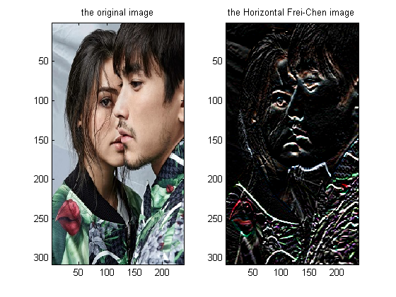
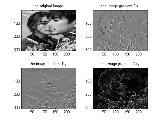
Image gradient
%# apply sobel filter on I with replicate padding
% sobelX and sobelY
Hx = [1 0 -1; 2 0 -2; 1 0 -1] ./ 8.0;
Hy = [1 2 1;0 0 0;-1 -2 -1] ./ 8.0;

% replicate padding
Ix = [im(:,1) im(:,1:end) im(:,end)];
Ixy = [Ix(1,:);Ix(1:end,:); Ix(end,:)];

% apply sobel filter with 2d-convolution and return results
% http://www.mathworks.com/help/matlab/ref/conv2.html
Dx = conv2(Ixy, Hx);
Dx = Dx(3:end-2,3:end-2);
Dy = conv2(Ixy, Hy);
Dy = Dy(3:end-2,3:end-2);
Dxy = sqrt(Dx.^2 + Dy.^2); % look like edges, right?

%# plot
figure;
subplot(2,2,1);
imagesc(im);
colormap(gray);
title('the original image');
subplot(2,2,2);
imagesc(Dx);
colormap(gray);
title('the image gradient Dx');
subplot(2,2,3);
imagesc(Dy);
colormap(gray);
title('the image gradient Dy');
subplot(2,2,4);
imagesc(Dxy);
colormap(gray);
title('the image gradient Dxy');