Calculating Path Sensitivity for Minefield Path Planning
CMSC498A - Independent Study
Summer and Fall 2002
Abstract
Path planning for minefields requires a consideration of risk and distance. Optimal paths through a minefield consider both factors. The sensitivity of a path indicates the likelihood of the path to change when mines are added or removed. This project studies the calculation and representation of path sensitivity. As a result of the experiments conducted in this study, we conclude that edges of a graph that are closer to the shortest path tend to be more sensitive, meaning that a change in these edges could result in a redirection of the shortest path. We found that shortest path edges tend to be sensitive to change in edge cost; these edges redirect with slight changes in cost.
Contents
Motivation (Top)
| The problem of minefield path planning requires better understanding of the sensitivity of shortest paths through minefields. Obviously, as the images in Figure 1 clearly depict, the failures of path planning through minefields have very destructive consequences. Therefore, an emphasis on correctness reflects the high priority of safety. |
Figure 1 |
Introduction (Top)
The Minefield Path Planning program computes a shortest path through a minefield, given the location of the mines. A grid of vertices represents the minefield. We can be add and/or remove the mines, which are located at a subset of vertices of the minefield. The number and proximity of mines near a vertex determine its risk value. Each vertex has 8 adjacent edges. All horizontal and vertical edges have equal length, and all diagonal edges have equal length. We compute the risk of an edge with a linear combination of the risk associated with the edge and the length of the edge. The cost associated with an edge equals the average of the risk associated with its two endpoints. The cost of a path is the sum of the costs of its edges. Of all the paths between S and G, the shortest path has the minimum cost. See Figure 2.
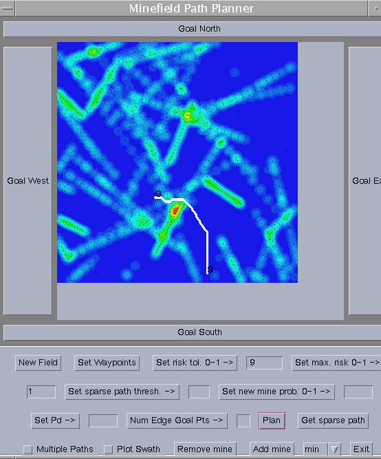
Figure 2
This research involves the sensitivity of the shortest path to changes in the minefield. In particular, as the cost of an edge decreases or increases, the shortest path may be redirected so that it either does or does not use this edge. Specifically, we study the maximum and minimum variations of edge costs such that the shortest path does not change, and we will discuss ways to represent this information. For a non-shortest path edge e, we want to know how much the cost of e must decrease before the shortest path redirects through e. Likewise, for a shortest path edge f, we want to know how much the cost of f must increase before the shortest path redirects through some edge other than f.
Glossary of Common Terms (Top)
Let G be a minefield graph and s and t be fixed vertices in G. Given an edge e of G, we define the following:
| alpha (a) | The lower tolerance of the edge that is e. This is the least cost e can have such that the shortest path does not pass through e. If the alpha value of edge e equals the cost of e, then the shortest path will never redirect through edge e. |
| delta-alpha(Da) | The cost of an edge minus its alpha value. This is the maximum amount that an edge's cost can decrease before the shortest path redirects through that edge. |
| beta(b) | The upper tolerance of an edge; that is, the greatest cost an edge can have such that the shortest path passes through this edge. |
| delta-beta(Db) | The cost of an edge's beta value minus the cost of the edge. The maximum amount an edge's cost can increase before the shortest path redirects through another edge. |
Observe that the a and Da values are most relevant for edges near the shortest path, and b and Db are most relevant for edges on the shortest path. In the next two sections, we consider each case in detail.
Non-Shortest Path Edges (Top)
For all non-shortest path edges, we know the value of b through intuition. No matter how much the cost of the edge increases, the shortest path between s and t will never redirect through e. Thus, for each non-shortest path edge, b = v.
With regards to non-shortest path edges, we are concerned with a and Da. We want to know how much the each edge e can decrease before the shortest path redirects through e. However, some edges cannot lie on the shortest path between s and t, even if the cost of such edges decreases to zero. For all edges that can never exist on the shortest path between s and t, the a value equals 0. Therefore, Da = the cost of the edge. We will not represent or analyze the sensitivity of such edges because they tend to be far away from the shortest path.
Computing a of non-shortest path edges - Naive Algorithm
Let P* denote the edges of the shortest path between two given vertices, s and t. The following algorithm computes a for non-shortest path edges:
for every non-shortest path edge e
cost(e) = 0
Let P' denote the new shortest path between s and t
a = cost(P*) - cost(P')
Restore the cost of e
|
This algorithm sets each non-shortest path edge to zero and checks if the shortest path redirects through the edge. Note that a = 0 when the cost of the new path equals the cost of the original path.
This algorithm has a poor running time. For every non-shortest path edge, we must perform the very costly operation of changing the edge cost twice. Also, we must perform the time-consuming computation of the shortest path once for every non-shortest path edge. In this application, our graphs will have thousands of edges. For example, a 200x200 grid has 320,000 edges and a 400x400 grid has 1,280,000 edges.
Neighborhood algorithm
The calculation of a for all non-shortest path edges clearly takes too much time. Therefore, we require a much faster algorithm. Either the number of edges to consider has to decrease, or the time to compute a for a single edge has to decrease. First we will analyze an approach that considers fewer edges.
In order to consider fewer edges, we must distinguish an edge that we will consider from an edge that we will not consider. Edges near the shortest path will most likely have interesting a values. Therefore, we can consider a "neighborhood" of edges near the shortest path from s to t. We define the neighborhood in Figure 3 as all edges that are adjacent to vertices of the shortest path. Thus, for each shortest path vertex, we consider seven non-shortest path edges.
Figure 3 û neighborhood defined by all edges adjacent to vertices of the shortest path. The blue edges represent neighborhood edges, and the red edges represent shortest path edges between s and t.
By considering the neighborhood edges, we greatly increase running time because we only consider a subset of all edges. Furthermore, this subset consists of edges that will likely have non-zero a values. In order to widen the scope of our analysis, we can redefine the neighborhood to include more edges, such as all edges that are two edges away from a shortest path vertex. However, this approach still does not solve the problem in a reasonable time because it requires too many shortest path computations. Therefore, we consider a faster approach that computes a for non-shortest path edges.
The ROC algorithm
The improved algorithm comes from the paper written by Ramaswamy, Orlin, and Chakravarti. In Theorem 3 of their paper, they outline an approach (herein known as the ROC algorithm) that requires only two shortest path computations to compute the a values for all non-shortest path edges of the grid. Their method capitalizes on the ability to look up the cost of the sub-path in an array of costs; thus, we can compute the shortest path to any vertex on the graph in constant time, given the root of a shortest path tree. This algorithm requires the computation of the two shortest path trees: one rooted at the source s and another at the goal t. Note that the previous algorithms only compute shortest path trees rooted at s. Therefore, the ROC algorithm requires one additional shortest path computation, the path rooted at t.
Here is the general procedure of the ROC algorithm. Let P* denote the edges of the shortest path between two given vertices, s and t.
for every non-shortest path edge e
"from" vertex = i
"to" vertex = j
Compute cost(s,i), cost(t,j), cost(s,j), and cost(t,i)
a = min( cost(s,t), cost(s,i) + cost(t,j), cost(s,j) + cost(t,i) )
|
Figure 4 provides a diagram of the situation inside each iteration of the for loop.
Figure 4
The computations of d(s,i), d(t,j), d(s,j), and d(t,i) simply require a lookup into the array which stores the cost information of the shortest path trees rooted at s and t.
The ROC algorithm easily surpasses the na´ve algorithm in terms of speed of computation. If the number of non-shortest path edges equals x, then the ROC algorithm requires 1/x as many additional shortest path computations. For example, given 472 shortest path edges, the na´ve algorithm requires 472 shortest path computations, in addition to the computation of the original shortest path. However, the ROC algorithm requires only 1 additional computation, which means it computes 1/472 as many shortest paths in our example. The ROC algorithm also considers all non-shortest edges, whereas the previous approach only considers the neighborhood of the shortest path. For example, one instance of the previous algorithm considers 7*n edges, where n is the number of vertices in the shortest path. However, the ROC algorithm considers (|E| - n - 1) vertices, where |E| equals the number of edges in the graph and n - 1 equals the number of edges in the shortest path (one less than the number of vertices).
In order to represent path sensitivity, we analyze the value of Da. For an edge e, we have Da = cost(e) - a. For the purpose of distinguishing edges of various sensitivity, we want edges with different Da values to have different colors; thus, we desire for the range of Da to map onto a range of colors. In order to effectively display the Da values of edges, we use a gray-scale coloring scheme, which contrasts well with the coloring scheme of the minefield. In order to focus the scope of our study, we do not color edges with Da = 0; such edges do not represent path sensitivity because the shortest path can never pass through.
A problem arises when we try to color edges because we can only color vertices (or other regions defined by x,y coordinates). Therefore, our scheme colors vertices according to surrounding Da values. Since each vertex has 8 adjacent edges, we offer the option of coloring vertices according to the minimum, average, or maximum of adjacent Da values. Although this coloring scheme fails to accurately represent the varying degrees of Da for edges, the 3 choices of coloring vertices will satisfy our need to representing path sensitivity.
In the gray-scale coloring scheme for Da, darker colors represent lower Da values, and lighter colors represent higher Da. Figure 5 shows a snapshot of the mine program with Da computed for all non-shortest path edges.
Figure 5
Shortest Path Edges (Top)
For each shortest path edge, we can easily determine a value because no matter how much the cost of the edge decreases, the shortest path does not redirect. However, changes in the shortest path may occur when a shortest path edge increases. The values of b and Db help us to understand the sensitivity of the shortest path edges to changes in cost. The value of b indicates how much the cost of the edge can increase such that the shortest path does not change. The value of Db represents the difference between the cost of b and cost of the edge; this value helps us to represent the path sensitivity of the shortest path edges, much like the value of Da helps us to understand the path sensitivity of non-shortest path edges.
Computing b of shortest path edges - Naive Algorithm
Let P* denote the edges of the shortest path between two given vertices on the grid. This approach computes b for all edges of P*:
for every edge e e P*
cost(e) = v
Let P' denote the new shortest path between s and t
b = cost(P') - cost(P*)
Restore the cost of e
|
The naive algorithm presented here differs from the naive algorithm of the previous section in two ways: First, this algorithm iterates over all shortest path edges, rather than all non-shortest path edges. Thus, the two algorithms analyze exclusive sets of edges. Second, we set each edge in this algorithm to infinity, essentially deleting it from the graph. Thus, the new shortest path must redirect through another edge.
However, like the na´ve algorithm for non-shortest path edges, this approach has a very slow running time because of the changes in the graph due to edge deletions. Hershberger and Suri offer an algorithm that computes b more efficiently.
The HS Algorithm
The improved algorithm (herein known as the HS Algorithm) comes from Theorems 1 and 2 in the paper by Hershberger and Suri. Like the ROC algorithm, the HS algorithm requires shortest path computations for the tree rooted at the source and for the tree rooted at the destination.
The HS algorithm proceeds by considering each edge (i,j) of the shortest path in succession. See Figure 6.

Figure 6
For each edge (i,j), we define a cut, which is an imaginary boundary between two shortest path vertices. See Figure 7.
Figure 7
In this diagram, we study all edges other than (i,j) that cross the cut; these edges (shown in red) have a "from" vertex u on the left side of the cut and a "to" vertex v on the right side of the cut. The new shortest path resulting from the deletion of edge (i,j) must cross the cut.
The algorithm requires the maintenance of the cut throughout our iteration over the shortest path edges. At all times, we must know all vertices that cross the cut because one of these vertices will lie on the shortest path. To maintain the cut, we use a min-heap of cost/edge pairs, ordered by cost. The cost component of each pair indicates the cost of the shortest path through the edge component, including the cost of the edge. The cost/edge pair of minimum cost indicates which edge we use from the cut for the shortest path.
Let P* denote the edges of the shortest path between two given vertices, s and t. This approach computes b for all edges of P*:
for every edge e e P*
Update the min-heap of cost/edge pairs
Let (u,v) represent the minimum cost edge which crosses the cut
Let P' denote the new shortest path between s and t through (u,v)
b = d(s,u) + d(u,v) + d(t,v)
|
Representation of b
Our solution to the problem of coloring shortest path edges resembles mirrors the problem we faced with coloring non-shortest path edges; we can color vertices, but not edges. Thus, as a solution, we color each shortest path vertex according to the minimum, average, or maximum of the two connected shortest path edges.
Our coloring scheme for shortest path edges ranges from red to yellow, with red representing lower Db values and yellow representing higher Db values. This scheme contrasts with the surrounding non-shortest path edges, which have a gray-scale coloring scheme. See Figure 8.
Figure 8 û Minefield before shortest path computation. The start and goal are circled.
Figure 9 û Minefield after shortest path computation. The small Db indicate that a slight change in an edge cost will redirect the shortest path.
Comparison of Algorithms (Top)
Ease of implementation
The first algorithm I implemented computed b values for shortest path edges using the na´ve approach. This implementation challenged me in the early stages largely because of my lack of familiarity with the program. Once I became comfortable with some of the code, the implementation of the algorithm proved to be simple.
Next, I worked on the na´ve algorithm for the a values of non-shortest path edges, and this task proved to be much easier than the previous one because of my understanding of how the Java classes interact. I was never able to fully test this algorithm because of the slow running time. My testing consisted of running the program and printing out useful information that allowed me to determine if the program is working correctly.
Third, I implemented the algorithm that computes a for a neighborhood of edges near the shortest path. Because the approach considers a small subset of all edges, I was able to run complete tests; however, I was only able to run complete and meaningful tests during lunch breaks because of the slow running time.
Fourth, I applied the ROC algorithm. This approach is very different from the na´ve approach, and thus, I wrote entirely new methods. I experienced moderate difficulty because I had to work with parts of the existing program that were unfamiliar.
Finally, I implemented the HS algorithm, which I found to be difficult. The maintenance of the cut proved to be the most challenging aspect. Also, the paper was a challenge to work through and fully comprehend.
Comparisons of Run Times and Experiments
Each experiment will have an image before the execution of the algorithms and an image after the execution of the algorithms. The output of the program will indicate the run time of each algorithm, and the analysis will compare the algorithms.
- Experiment 1: The start and goal are on either side of a mine.
- Experiment 2: The start and goal points are on either side of an area with a heavy concentration of mines.
- Experiment 3: The start and goal points lie on opposite corners of the minefield.
Experiment 1: The start and goal are on either side of a mine. See Figure 10.
Figure 10 û The start and goal points are on either side of a mine.
HS Algorithm (shortest path edges) and ROC Algorithm (non-shortest path edges)
| Begin find betas... | Fri Dec 06 16:00:30 EST 2002 |
| END find betas... | Fri Dec 06 16:00:31 EST 2002 |
| Begin find alphas... | Fri Dec 06 16:00:31 EST 2002 |
| END find alphas... | Fri Dec 06 16:00:33 EST 2002 |
Naive Algorithm (shortest path edges) and Neighborhood Algorithm (non-shortest path edges)
| Begin find betas... | Fri Dec 06 16:11:54 EST 2002 |
| END find betas... | Fri Dec 06 16:11:58 EST 2002 |
| Begin find alphas... | Fri Dec 06 16:11:58 EST 2002 |
| END find alphas... | Fri Dec 06 16:12:43 EST 2002 |
Figure 11 û After planning the shortest path and representing path sensitivity.
Analysis
The white points represent the shortest path vertices. The red blocks represent the sensitivity of the shortest path vertices. The red color indicates a small Db value; therefore, a small increase in the cost of the edge will redirect the shortest path. The gray-scale colors represent the sensitivity of the non-shortest path edges that could lie on the shortest path with a change in cost. The edges closer to the shortest path require a small decrease in cost to redirect the shortest path; hence, these edges are dark gray. The edges further from the shortest path require a greater decrease in cost to redirect the shortest path; hence, these edges are lighter gray.
Experiment 2: The start and goal points are on either side of an area with a heavy concentration of mines. See Figure 12.
Figure 12 û The start and goal points are on either side of an area with a heavy concentration of mines.
HS Algorithm (shortest path edges) and ROC Algorithm (non-shortest path edges)
| Begin find betas... | Fri Dec 06 16:27:42 EST 2002 |
| END find betas... | Fri Dec 06 16:27:43 EST 2002 |
| Begin find alphas... | Fri Dec 06 16:27:43 EST 2002 |
| END find alphas... | Fri Dec 06 16:27:45 EST 2002 |
Naive Algorithm (shortest path edges) and Neighborhood Algorithm (non-shortest path edges)
| Begin find betas... | Fri Dec 06 16:33:08 EST 2002 |
| END find betas... | Fri Dec 06 16:33:24 EST 2002 |
| Begin find alphas... | Fri Dec 06 16:33:24 EST 2002 |
| END find alphas... | Fri Dec 06 16:35:47 EST 2002 |

Figure 13 û After planning the shortest path and representing path sensitivity.
Analysis
Note the orange color of the shortest path edges near the middle of the path. This coloring indicates that the shortest path will redirect away from these edges only with a relatively high increase in edge cost. Also, note the dark coloring of some of the edges far from the path. A small decrease in the cost of these edges would cause a major redirection of the shortest path.
Experiment 3: The start and goal points lie on opposite corners of the minefield. See Figure 14.
Figure 14 û The start and goal points lie on opposite corners of the minefield.
HS Algorithm (shortest path edges) and ROC Algorithm (non-shortest path edges)
| Begin find betas... | Fri Dec 06 16:49:11 EST 2002 |
| END find betas... | Fri Dec 06 16:49:13 EST 2002 |
| Begin find alphas... | Fri Dec 06 16:49:13 EST 2002 |
| END find alphas... | Fri Dec 06 16:49:15 EST 2002 |
Naive Algorithm (shortest path edges) and Neighborhood Algorithm (non-shortest path edges)
| Begin find betas... | Fri Dec 06 16:53:06 EST 2002 |
| END find betas... | Fri Dec 06 16:53:55 EST 2002 |
| Begin find alphas... | Fri Dec 06 16:53:55 EST 2002 |
| END find alphas... | Fri Dec 06 17:01:09 EST 2002 |
Figure 15 û After planning the shortest path and representing path sensitivity.
Analysis
The distance between the start and goal vertices does not greatly affect the combined running time of the faster algorithms. This experiment runs only one second slower than experiments one and two. However, in this experiment, the slower algorithms run over three times slower than experiment two and eight times slower than experiment one.
Sources (Top)
Hershberger, John and Subhash Suri. "Vickrey Prices and Shortest Paths: What is an edge worth?" http://www.cs.ucsb.edu/~suri/psdir/vickrey.ps 2001.
Piatko, Christine D, Christopher P. Diehl, Paul McNamee, Cheryl Resch, and I-Jeng Wang. "Stochastic Search and Graph Techniques for MCM Path Planning." Proceedings of the SPIE. Vol. 4742. April 2002.
Ramaswamy© Ramkumar, James B. Orlin, and Nilopal Chakravarti. "Sensitivity Analysis for Shortest Path Problems and Maximum Capacity Graph Problems in Undirected Graphs." http://web.mit.edu/jorlin/www/papersfolder/SAabstract.html
Ramilingham, G. and Thomas Reps. "An Incremental Algorithm for a Generalization of the Shortest-Path Problem." Journal of Algorithms. Vol. 21, No. 2. 267-305. 1996.
Resch, Cheryl, Christine Piatko, Fernando Pineda, Jessica Pistole, and I-Jeng Wang. "Path Planning for Mine Countermeasures." 2002.
Other Formats
MS Word Version