Case Study: Gaining Insight into Markov Chains by Using Monte Carlo Simulations
David Rouff
As we studied in Unit IV, Monte Carlo simulations help provide answers for problems too complicated to solve explicitly/in closed form. In science, these types of problems weren’t even considered much more than 100 years ago because they were simply too complicated to think that they were solvable.
About 100 years ago, A Russian mathematician named Andrey Markov published an insight into probability that allowed us to define probability relationships between the previous state of a system and the current state. In doing so, he linked probability to time and enabled us to calculate the probability of a chain of dependent events. As can be expected, adding the time dimension to probabilities of systems can become very complicated very quickly, so the field did not advance past nominally sized systems until information technology enabled large numbers of calculations to be performed and stored. Markov chain systems can still grow tremendously big, however, and solving these systems is one application area of Monte Carlo simulations.
Definitions
The simplest of probability examples (flipping a coin) will help to introduce the definition of a Markov Chain. The probability that it comes up heads is ½ and the probability that it comes up tails is also ½. This can be written as a vector consisting of the probabilities for the different outcomes.
H T
V(coin)=[ ½ ½ ]
Likewise, for rolling a die:
1 2 3 4 5 6
V(die)=[ 1/6 1/6 1/6 1/6 1/6 1/6 ]
It does not make much sense with coins and dice to consider that the current state has any impact on the future state, if the last flip of a coin was heads, the next flip is just as likely to be heads as tails. Each flip is an independent event. For many systems, however, there is an impact of the current state on the next state. The frequently used example is the weather. Tomorrow’s forecast is impacted by today’s weather.
Suppose the only 2 weather conditions are sunny and cloudy, and that tomorrow’s weather is twice as likely to be the same as today’s weather as it is to change. Then the probability vector of sun or clouds tomorrow is not the same as the vector for flipping a coin, but rather is:
Different from Today Same as Today
V(Weather)=[ 1/3 2/3 ]
To be more exact, consider the probability vector of each current state:
Tomorrow: Sunny Cloudy
V(Sunny Today) = [ 2/3 1/3 ]
V(Cloudy Today) = [ 1/3 2/3 ]
The link between the current state and the probability for the next state defines a Markov Chain. Joined together, the probability vectors of each possible current state create a Transition Matrix.
In a “what have you done for me lately” sense, the impact of previous time steps are not considered. It does not matter how remote of a chance it was that the system got to where it is, because it is there as the Markov Chain’s starting point. The looking at the state of a system past the next time step, however, is a key part of analyzing Markov Chains.
The probability for 2 steps out is the product of probabilities. Continuing with the nominal weather example, the weather in two days is the product of the weather states for each. For example, Starting with a Sunny Day as the current state, the probability that it will be Sunny in 2 days is the probability that it stays sunny tomorrow (2/3) * probability that it stays sunny the next day(2/3) added to the probability that it changes to Cloudy (1/3) * the probability that it changes back to sunny (1/3). Restated, given that it is Sunny today, the probability of sun in 2 days =2/3*2/3+1/3*1/3.
Likewise, starting with Sunny at time zero, the probability of Cloudy at time 2 is 2/3(Sunny Tomorrow)*1/3(changing to Cloudy after tomorrow) + 1/3(changing to Cloudy Tomorrow)*2/3(staying cloudy after tomorrow). An easier way to understand and calculate the probability vector for 2 time periods out is simply the probability vector times the transition matrix. To do all probability vectors simultaneously, the calculation is simply raising the matrix to a power.
In many Markov Chains, a measure of independence is regained after several time steps as the probabilities of future states even out to constant numbers across all of the starting states. After N time steps, the probability of being in a state is independent of the starting state. When this happens, the system is said to have reached equilibrium. In the simple weather system, the transition matrix very quickly evens out as seen below, where the matrix P(j) gives the probabilities that the weather j days from now will be sunny or rainy, given that today is sunny (first row) or rainy (second row):
P(1) =
0.33333333333333 0.66666666666667
0.66666666666667 0.33333333333333
P(2) =
0.55555555555556 0.44444444444444
0.44444444444444 0.55555555555556
P(3) =
0.48148148148148 0.51851851851852
0.51851851851852 0.48148148148148
P(4) =
0.50617283950617 0.49382716049383
0.49382716049383 0.50617283950617
Here the chance of sun 4 days after a cloudy day is getting very close to the chance of sun 4 days after a cloudy day. In a similar fashion, we saw an example of using a number of time steps to gain independence from a starting point in the challenge of counting dimer configurations (Chapter 18). Each lattice was connected to the next lattice by the probabilities of adding, deleting, or rotating dimers. But the dependence diminished after several time steps so that the lattice configurations that were counted were independent of each other.
Consider the constrained weather system defined below. Each day can be Sunny, Windy, Cloudy, or Rainy. The wind needs to blow in order to blow clouds in or out, and clouds need to be present in order to rain. So, the Markov Chain’s transition matrix is:
|
|
Sunny |
Windy |
Cloudy |
Rainy |
|
Sunny |
0.5 |
0.5 |
0 |
0 |
|
Windy |
0.333333 |
0.333333 |
0.333333 |
0 |
|
Cloudy |
0 |
0.333333 |
0.333333 |
0.333333 |
|
Rainy |
0 |
0 |
0.5 |
0.5 |
There is no direct way to go from a Sunny day to a Cloudy or Rainy day in 1 time step, so the top row of the transition matrix has zeros in the last 2 columns. Despite this, the system can still reach an equilibrium that includes average values for each state of the weather.
P(1) =
0.5000 0.5000 0 0
0.3333 0.3333
0.3333 0
0 0.3333
0.3333 0.3333
0 0 0.5000 0.5000
P(29) reaches equilibrium to 4 decimal places with
0.2000 0.3000
0.3000 0.2000
0.2000 0.3000
0.3000 0.2000
0.2000 0.3000
0.3000 0.2000
0.2000 0.3000
0.3000 0.2000
Frequently the task is not just to derive the probabilities, but to also show sample patterns of activity. For the weather system above, one way to simulate the weather for a period of N days is given by the algorithm:
function
exampleWeather()
%This program performs a
Monte Carlo on the 4-state weather Markov Chain.
N=14;
P=[1/2 1/2 0 0
1/3 1/3 1/3 0
0 1/3 1/3 1/3
0 0 1/2 1/2];
% This algorithm produces
a matrix showing the simulated weather for a month.
% The first day is T=1, and
Sunny
fprintf(1,'Day Sunny Windy Cloudy Rainy \n');
Weather(1,:)=[1 0 0 0];
fprintf(1,'
1 - %1d %1d
%1d %1d \n',Weather(1,:));
for
t=1:N
TomorrowVector=Weather(t,:)*P;
% The probability vector sums to 1, so the following
randomize and
% select statements simulate the occurrence of each type
of weather
% following the transition matrix P above.
Today=rand();
switch true
case
Today <= TomorrowVector(1)
Weather(t+1,:)=[1 0 0 0];
case Today <=
(TomorrowVector(1)+TomorrowVector(2))
Weather(t+1,:)=[0 1 0 0];
case Today <=
(TomorrowVector(1)+TomorrowVector(2)+TomorrowVector(3))
Weather(t+1,:)=[0 0 1 0];
otherwise
Weather(t+1,:)=[0 0 0 1];
end %switch
fprintf(1,' %2d -
%1d %1d %1d
%1d \n',t+1, Weather(t+1,:));
end %for
t
The output can be verified as:
Day Sunny Windy Cloudy Rainy
1 - 1 0 0 0
2 - 0 1 0 0
3 - 1 0 0 0
4 - 1 0 0 0
5 - 1 0 0 0
6 - 0 1 0 0
7 - 0 1 0 0
8 - 1 0 0 0
9 - 0 1 0 0
10 - 0 1 0 0
11 - 0 1 0 0
12 - 1 0 0 0
13 - 1 0 0 0
14 - 0 1 0 0
Note that the probability shows the average over a long period of time while the sample pattern of activity shows all sunny days and windy days when started with a sunny day.
Absorbing Chains
An important phenomena in Markov Chain analysis is the existence of a state that is inescapable once reached. A chain is called an Absorbing Markov Chain if it eventually leads to a solution that stays fixed. Transitional states have probabilities that the system will go to different states, once reached, the probability for the next state from a fixed one is 0 and the probability to stay in the current state is 1.
For a nominal and slightly morbid example, consider the simple Markov Chain transition matrix giving the probabilities that Bob is alive or dead. Given that Bob is alive at the start, assume the probability that he dies tomorrow is 0.000043.
Bob’s Transition Matrix
Tomorrow:
alive dead
V(Alive) [ .999967
.000043]
V(Dead) [
.000 1.0 ]
The good news for Bob is that the chance he’s doomed today is very remote. The bad news is that the example was made to give a definition of an “absorbing chain,” so sooner or later the system will be ‘absorbed’ into the state and stay there permanently… (Sorry Bob). Albeit small, there is a chance that Bob will be dead tomorrow, and once he’s dead, there is no chance of him coming back.
CHALLENGE 1. Part 1a: Bob’s Life does not make a very interesting transition matrix, but does give a chance to ask the more interesting question of, “How long will Bob live?”
Without
some magical method to determine Bob’s life expectancy immediately from the
transition matrix, the only way to tell Bob how many days he has is to simulate
Bob’s life repeatedly counting days, until the absorbing state is reached. Since that may happen on the first day, or not
for many, many years, the best answer is the average of many such Monte Carlo
simulations. Run a Monte Carlo
simulation for Bob’s life to give an average life expectancy.
1b. Truncate the probability to 4 decimal places
(i.e., .9999) and re-run the simulation.
What is the impact to Bob’s life of the 0.000067 that was truncated?
1c. Maybe we can help Bob out and get a more precise calculation in the process. The next part of this challenge is to redo the calculation to predict the exact split-second of Bob’s demise instead of just the year. Also, add a counter that prints out Bob’s Age every time he enters a new year while the experiment is working. (Before starting the program, refresh your memory with how to interrupt a program’s execution (i.e., CTRL/Break).) After the program has run for a few minutes, or perhaps when Bob passes into unreasonable ages, skip to the next part.
1d. Bob will be tickled to see his longevity, but he may be somewhat deflated when he reads your reply to this part of the challenge. Explain why the program does not stop running. Is Bob really immortal, or is there a computational reason that the absorbing state is not reached (Hint: review part 1 of this text)?
POINTER: The key for Bob’s longevity leaves the topic of Markov Chains somewhat, but is worth iterating a key point related to Part 1 of the text. Choosing the unit of measure for performing the most accurate calculation possible is an optimization problem similar to the basic law of supply and demand chart. Larger units of measure will suffer much less round-off error, but will give a less precise answer because the calculations are performed with the larger units.
Very
small units of measure could give a more precise answer, but cause the
algorithm to work through many more iterations (864,000 tenths of seconds in a
day). Tiny units also become prone to
round-off error as the elements of calculations span past the 15 significant
digits that floating point data structures can hold.
Another frequently used Markov Chain is that of a random walk. In a random walk, the subject, lets say its Bob again, decides which way to walk at the end of each block on a 7-block long street. If the Bob reaches the house at either end of the street, he goes inside and the walk is over. The transition matrix for this random walk is similar to the weather described above:
|
|
Block 1 |
Block 2 |
Block 3 |
Block 4 |
Block 5 |
Block 6 |
Block 7 |
|
Block 1 |
1 |
0 |
0 |
0 |
0 |
0 |
0 |
|
Block 2 |
0.5 |
0 |
0.5 |
0 |
0 |
0 |
0 |
|
Block 3 |
0 |
0.5 |
0 |
0.5 |
0 |
0 |
0 |
|
Block 4 |
0 |
0 |
0.5 |
0 |
0.5 |
0 |
0 |
|
Block 5 |
0 |
0 |
0 |
0.5 |
0 |
0.5 |
0 |
|
Block 6 |
0 |
0 |
0 |
0 |
0.5 |
0 |
0.5 |
|
Block 7 |
0 |
0 |
0 |
0 |
0 |
0 |
1 |
Lucky for Bob, the absorbing states in this chain are just the act of reaching the house on either end of the street.
CHALLENGE 2: Part 2a. Starting at block 4, tell how long on average a random walk will last. 2b. Give the block by block output for a random walk in a chart similar to the weather for a month as described above.
Canonical Form
In analyzing Absorbing Markov Chains, it is useful to put them into a standard form that groups the transient states to the top left and the absorbing states to the bottom right. The absorbing states take on the form of the identity matrix, with zeros to the left and the probabilities to reach each absorbing state in the top right corner above the identity. The rest of the matrix is the collection of temporary, “transient” states in the top left
Transient | Remainder
Zeros | Identity
The random walk transition matrix in this form is:
|
|
Block 2 |
Block 3 |
Block 4 |
Block 5 |
Block 6 |
Block 1 |
Block 7 |
|
Block 2 |
0 |
0.5 |
0 |
0 |
0 |
0.5 |
0 |
|
Block 3 |
0.5 |
0 |
0.5 |
0 |
0 |
0 |
0 |
|
Block 4 |
0 |
0.5 |
0 |
0.5 |
0 |
0 |
0 |
|
Block 5 |
0 |
0 |
0.5 |
0 |
0.5 |
0 |
0 |
|
Block 6 |
0 |
0 |
0 |
0.5 |
0 |
0 |
0.5 |
|
Block 1 |
0 |
0 |
0 |
0 |
0 |
1 |
0 |
|
Block 7 |
0 |
0 |
0 |
0 |
0 |
0 |
1 |
The ‘interesting section’ of this matrix is the transient blocks. For an Absorbing Markov Chain, the fundamental matrix is defined as the inverse of the Identity minus this section of the matrix.
p=[
0 0.5 0 0 0
0.5 0 0.5 0 0
0 0.5 0 0.5 0
0 0 0.5 0 0.5
0 0 0 0.5 0
]
FundamentalMatrix=(eye(5)-p)^(-1)
1.6667 1.3333 1.0000 0.6667 0.3333
1.3333 2.6667 2.0000 1.3333 0.6667
1.0000 2.0000 3.0000 2.0000 1.0000
0.6667 1.3333 2.0000 2.6667 1.3333
0.3333 0.6667 1.0000 1.3333 1.6667
This fundamental matrix for the chain gives the approximate number of time steps that that will be spent in each state before being absorbed. To get a total of the time before being absorbed for each starting point, sum the row. I.e., starting at Block 1, the average total time before being absorbed is 1.6667 + 1.3333 + 1.0000 + 0.6667 + 0.3333 = 5. The average time before being absorbed starting from block 4 is 9. Compare this with your answer to the previous challenge.
CHALLENGE 1e. Returning to the first Challenge, use the canonical form and fundamental matrix to calculate the average length of Bob’s life directly. Compare this with your answer to the first challenge.
Markov Chain analysis is commonly used to answer questions such as how long the transitional states will last, what all of the states are, and what the probability is for eventually ending up in each of the absorbing states. The previous examples and challenges have been purposefully trivial. Larger or more complicated systems become difficult if not impossible without Monte Carlo techniques. The next 2 challenges show why Monte Carlo simulations are used to approximate solutions to larger Markov Chain systems.
CHALLENGE
3: First, expand the random walk from back and forth on a street, to a random
walk through a 2 dimensional grid, i.e., Manhattan-like city blocks.
Without
a compass or road signs, Bob becomes analogous to a blind rat in a maze. Assuming an 8x8 chessboard sized city, where
the walker is equally likely to walk in any 4-connected direction (not
diagonally) at any block, answer the same questions about the duration and
example path of the random walk. Give
Bob a starting point of square (1,1) and make his target square (8,8). Create an animation of the Monte Carlo
simulated path (since the state space is a matrix, it becomes too lengthy to
repeatedly print the matrix at the command line).
This
space is still nominally sized compared to real world systems, but it has 64
possible states. With the state space
having N squared states, the space becomes unmanageable as N grows. The direct calculation of the average
duration in transient states involves the inverse of a matrix. From earlier in the semester, we know this
is not an easy, or accurate computation in more complicated matrices. The Monte Carlo Simulation appears to be a
better method to approximate the system’s transient duration.
Hint: Rather than define and store the complete transition matrix, it is easier to calculate the transition probability each time based on the current location.
An example output from the animation above could look like this figure:
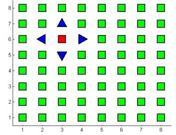
Figure: Chessboard with Random Walker in Red and possible moves shown as blue triangles.
POINTER: One of the special purpose jigsaws of the
scientific computing toolbox is to solve a hard problem by breaking it into a
series of easy problems. Recursion and
homotopy (part 6 of the text) are obvious examples. The challenge above introduces a different way to decompose a
harder problem. Consider a random walk
over a 1000 by 1000 grid, or a random walk over an unbounded plane. Markov’s probability transition matrix
becomes super large. Since most of the
probability elements are zero, the computation could be improved by concepts in
part 7 of the text (working with sparse matrices), but an alternative for this
type of problem is the concept of decomposing a big problem into ‘local’
computations. For the random walk, no
matter where the walker is, there are only 4 elements he could move into. The probability of all other locations is
zero. So, rather than the ‘global’
computation across the entire map, the challenge instructs to generate a
‘local’ computation based on the walker’s current position.
CHALLENGE
4: The final challenge is a simulation of a problem known as a ‘stepping stone’
where different plants are competing for space (sunlight and soil) across a
bounded plain.
In
this simulation, 4 types of plants are equally suited for survival, and in
competition with each other for space in a homogenous environment. To make this problem programmable, the
environment is divided into a chessboard similar to the random walk, and limit
the environment to having only one plant per square. Also, to make the environment more homogeneous, where every cell
has an equal amount of adjacency, define the top row as adjacent to the bottom
row and the left edge adjacent to the right edge. Topologically, this changes the surface into a torus.
The
state space starts out with an even distribution of each plant randomly spread
across the region.
The
plants compete with each other in the following manner: Randomly, the plant in
one square will send shoots that grow and take over one of the 4-adjacent
areas.
This
stepping stone is proven to converge to a single plant species winning, but it
may take a long time to complete at the 8 by 8 size, so start with a map hat is
4 by 4. Plot the space so it can be
observed, run a simulation to watch the competition unfold.
HINT:
While the rules above are relatively easy to define, the Markov Chain for this
system would be prohibitively large to store.
Hence, the Monte Carlo simulation becomes the preferred way to analyze
the system. As in the random walk, this
is easiest to program by picking one cell at a time, then randomly picking the
adjacent location to take over.
References
Markov chain Monte Carlo From Wikipedia, the free encyclopedia
http://en.wikipedia.org/wiki/Markov_chain_Monte_Carlo
Markov Chain -- from Wolfram MathWorld
http://mathworld.wolfram.com/MarkovChain.html
Grinstead, Charles M. and Snell, J. Laurie. Introduction to Probability. Second Revised Edition, July 1997.
Walpole, Ronald E. and Myers, Raymond H. Probability and Statistics for Engineers and Scientists. 4th Edition Macmillin:1989.
Russell, Stuart and Norvig, Peter. Artificial Intelligence: A Modern Approach. 2nd Edition. Prentice Hall: 2003.