
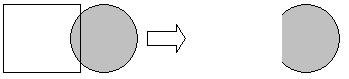
2. If the sphere is partially overlapping the "square" but not the corners. It will be displayed improperly.
Independent Research Project
Author: Aleksey Martynov
Faculty Advisor: Dr. David Mount
Date: May 2000
ABSTRACT
The paper discusses a new algorithm for performing ray-object intersection. These intersections are used extensively in ray tracing algorithms. The goal of the new algorithm is to minimize the rendering time by improving the average time of the ray-object intersection tests. The algorithm focuses on rendering spheres and presents spheres in 4-dimensional (sphere) space in order to optimize the structure of the resulting data structure for searching purposes. The results of the algorithm are compared against simple brute-force search method and enhancements to the algorithm are discussed.
Introduction
Ray tracing is a technique for rendering realistic images of 3-dimensional scenes. The image is generated by determining a color of every pixel in the picture. Imaginary rays are extended originating at the eye of the viewer and going through every individual pixel. The ray is tested against the objects in the scene and the closest intersecting object is found. At the point of intersection, surface normal, visibility of the light sources, ambient light, color of the objects surface and other parameters determine the color of the pixel. Additional reflection and refraction rays could be also extended in order to improve the realism of the picture. In case the ray does not hit any object in the scene, some preset background color is set to the pixel.
One of the problems with ray tracing algorithms is the rendering time. Since every pixel in the picture needs to be tested with an appropriate ray, there is a large number of ray-object intersections that need to be performed. For every ray in the picture, the search through the scene needs to be performed in order to determine the first object that is hit by the ray. Since there could potentially be thousands of objects in the scene, every search can take extensive time, and the necessity to perform the search for every pixel complicates the problem even further.
The goal of this project is to produce a new faster method for rendering realistically looking images of spheres in space. There are a number of potential applications for such a package; one application that the project specifically focuses on is rendering molecules. In rendering molecules, an image may consist of a large number of spheres, anywhere from couple of hundred to thousands.
The high-level idea behind this project is to conduct
ray-object intersection tests in a space that is higher then 3D. A sphere
can be uniquely represented by 4 coordinates: x, y, and z coordinates of
the center of the sphere and r (radius) of the sphere. The natural way
to represent spheres is then as points in 4 space, where the base coordinates
are x, y, z, and r. Then we can store spheres in a hierarchical subdivision
of 4 space, and conduct the ray-object intersections according to the new
partitioning of the space. The advantage that this method provides is the
fact that it allows to partition a set of spheres based on a larger number
of parameters (4), therefore make pruning of the search tree more effective.
Definitions
Before we discuss the algorithm itself, some of the terms must be defined.
A Point in primal space maps to a point in dual space with r-coordinate set to 0 (or a sphere with radius 0). The algorithm does not use this mapping at this point, however it can be potentially used in the future to determine the point of intersection between the ray and the sphere.
A Sphere in primal space maps to a point in dual space. This mapping is the one that allows algorithm to treat spheres as points and build the data structures based on that fact. The nodes in the new data structure include all the points in dual space, which fall within a particular condition.
A Ray in primal space maps to a region in dual space such that it divides dual space into two parts: inside the region and outside the region. The inside space must include all the points that represent the spheres in primal space that the ray intersects. The outside region includes all other points.
Outline of the Algorithm
The idea behind the algorithm is that given a list of spheres, a kd-tree will be created, which discriminates on 4 coordinates (x, y, z of the center and radius) as opposed to just 3 coordinates regularly used in spatial data structures. That tree will provide a better distribution of the spheres throughout the tree, and will allow making searches through the tree more efficient by allowing to "prune" more nodes that do not have to be visited. Below is a more detailed outline of the algorithm.
[XRmin - XRmax + 2 RRmax]
[YRmin - YRmax + 2 RRmax]
[ZRmin - ZRmax + 2 RRmax]
Improvements to the Algorithm
Prescan Technique
One of the possible improvements to the algorithm is prescan technique. The idea behind this technique is that instead of shooting a ray through every pixel in the picture, program will shoot 4 rays through the corners of a "square" of pixels, the size of which is predefined by some PIXEL_STEP. If all 4 rays do not hit any sphere, fill all the pixels in the "square" with the background color and assume that all the rays through the region will not intersect any sphere. If all 4 rays hit the same sphere, assume that all the rays through the "square" hit the same sphere and calculate pixel colors based on that assumption. If at least one of the rays hits a different sphere, shoot rays through every pixel in the "square" in order to render the appropriate colors.
The advantage of the algorithm is that it produces a significant speedup in rendering time, especially in case of scenes with large objects close to the eye location or significant amounts of "open" space. In addition, by increasing PIXEL_STEP, rendering time can be improved.
However, this improvement technique also presents certain disadvantages, which may cause some pixels to be rendered improperly. In addition, larger PIXEL_STEP may result in worse quality of the final image.
Consider following scenarios:
Current Implementation
The current implementation of the algorithm is done in Microsoft Visual C++ 6.0 in Windows NT 4.0 environment. Microsoft Foundation Classes (MFC) are used in the implementation to provide user interaction with the user and display the output. The program takes text file as input. The input file contains information about position of the camera (eye location, direction, and orientation of the viewing frame), position and properties of the lights in the picture, characteristics of the surfaces assigned to objects, and finally the list of all the spheres in space.
The current program does not implement reflection or refraction of the rays. However, shadows are implemented. The main goal of this implementation is to provide means for comparing the running time of the algorithm versus brute force implementation. Therefore implementation of additional complexity in shooting reflection/refraction rays is not necessary, since it will not affect the comparative result. The user interface for the current implementation can be seen in Figure 1 below.
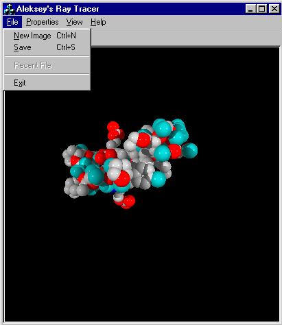
Figure 1: Windows User Interface
The interface allows user to select the method of creating the image (either Brute Force, 4D Tree, or PreScan Method). The user then creates a new image from an input file. In this implementation, the image is created to have 400 by 400 pixels dimensions. However, in the future implementations, the arbitrary size of the window is desirable.
The implementation keeps track of some information necessary to perform the analysis on the algorithm. Information stored includes the number of spheres in image, the time necessary for the creation of the image, the number of ray-sphere intersection tests actually performed, and the name of the input file. The information is stored for all the images created during the run of the program and it can be viewed and stored at any time.
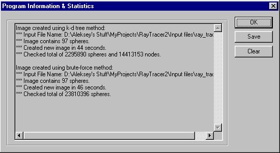
Figure 2: Program Information Screen
Experimental Results
Number of experiments were conducted with the current implementation of the algorithm. The main goal of the experiments was to analyze the growth of the rendering time as the number of spheres in the scene increases.
Three different algorithms were tested with the same data:

Figure 3: Creation time vs. Number of Spheres Graph
The creation time in all the figures refers to the time measured from the moment the input file is specified and until the final image is created. As can be seen from the graph, the creation time for brute force (red) algorithm rises at a much steeper rate then that for 4D Tree (blue) or Pre-Scan (yellow) methods. The Pre-Scan method has better creation time then the 4D Tree algorithm, however that difference is constant and is not as significant in the overall performance of the algorithm as the difference between brute force and 4D Tree.
The graph shown in Figure 3 shows that both 4D Tree and Pre-Scan algorithms produce better rendering times then the brute force method for number of spheres exceeding 100 spheres. The large number of spheres results in the longer rendering times. However, it is logical to suspect, that for some smaller number of spheres brute force method should provide better results, since there is no overhead for building a tree or traversing the tree as opposed to 4D Tree method. Another experiment was conducted in order to determine at what number of spheres does the 4D Tree algorithm becomes more efficient then the brute force method. Results of this experiment can be seen below in Figure 4.
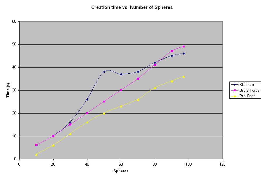
Figure 4: Creation Time vs. Number of Spheres Graph
This graph shows that initially the brute force algorithm produces better results than the 4D Tree algorithm. As mentioned before, this is explained but the fact that 4D Tree algorithm requires creation of a data structure, which increases the overhead. However, once the number of spheres exceeds 80 to 100 spheres, the 4D Tree starts to show better results. It is interesting to note that the Pre-Scan method cuts the overhead cost by not using the tree at every step of rendering, therefore the creation time for the Pre-Scan method is better. The interesting shape of the line for the KD Tree results is explained only by the fact that the particular sample the experiment was conducted on has that property. The shape is not at all representative of any specific feature of the new algorithm.
Pre-Scan Method Issues
As discussed previously in the section on the Pre-Scan method, some errors can occur in rendering of the final image. It is interesting to see how those errors affect the overall quality of the image and whether they play significant role in the final image. In Figure 5 below, one can see the image created without using Pre-Scan method, where every pixel in the picture is rendered by finding an appropriate ray-sphere intersection.
Figure 5: Image of a fragment of the T4 lysozyme created using 4D Tree method
As one can see, the image is rendered properly (no anti-aliasing implemented). However, on the same scene created with the Pre-Scan method, some imperfections can be found, as seen in Figure 6.
Figure 6: Image of a fragment of the T4 lysozyme created using Pre-Scan method
The differences on the image in Figure 6 are the same as predicted by the analysis of the optimization. Certain pixels are assigned incorrect colors. However, the differences are relatively insignificant and are not easily found. The images created with the Pre-Scan method show the information necessary for correctly identifying all the important of the image, and since those images are created faster, this method proves valuable for generating preview images or images which are not going to be analyzed in great detail. If the image must contain no imperfections, 4D Tree method should be used, which still provide better rendering time than the regular brute force method.
Discussion
The experimental data shows that the new algorithm provides significant improvement in rendering time over the brute force method for a large number of spheres. As expected with any complicated data structure, the initial creation time is longer, since the program needs to construct the data structure before using it. In addition, traversing the data structure can take longer than simply traversing a list, as is the case of the brute-force method. These facts account for the results of the experiments when less then 100 spheres were rendered in the scene. For a small number of spheres (Figure 4), the brute-force algorithm exhibits the same if not better rendering time. However, for the scenes involving over 100 spheres, the 4D algorithm is clearly better. For a large number of scientific applications, such as rendering molecules, scenes involving thousands of spheres representing atoms are not uncommon. The new algorithm provides means for fast rendering those images. The Pre-Scan improvement to the algorithm allows the user to preview the final image in shorter time, before rendering the final image.
The important fact to note about the 4D algorithm is that the tree is constructed only once and can be then reused to produce images of the scene from any location of the camera. This advantage improves overall rendering time, for the tree creation time only factors into the first image, and all the consecutive images created using either full algorithm or pre-scan method can be created using the same data structure.
The relative success of the algorithm opens a possibility for representing other objects in 3-dimensional space as objects in higher spaces in order to build more efficient data structures and ultimately improve the algorithmic running times. Better parsing of the object set into different nodes in the data structure, if done correctly, should translate into faster search times through the data structure. Different mappings could be derived for more complicated object then spheres, such as cubes or prisms for example. More work needs to be done in order to determine if this is a promising direction.
Conclusion
The 4D Ray tracing algorithm is developed to improve rendering times for the scenes involving large number of spheres. The algorithm builds its data structure for storing spheres by mapping spheres into regions in 4-dimensional space, specified by x, y, z coordinates of the center of the sphere and the radius of the sphere as the fourth coordinate. A number of experiments performed on the different data sets show that the algorithm provides significant improvement in rendering time over a brute-force search method. The data also shows that rendering time does not grow as fast as that for brute-force algorithm as the number of spheres increases.
Suggestions for Future Research
The next step in developing the algorithm is to compare
the rendering time of the algorithm to rendering times of the current efficient
implementations of ray tracing algorithms. It is important to see whether
the new algorithm compares favorably to the implementations that utilize
efficient 3-dimensional data structures. The algorithm can be improved
by introducing better search techniques through the data structure and
by optimizing the code of the application. Additionally, future researchers
could address issue of coherence. Coherence refers to the fact that since
the next ray is shot very close to the previous one, it is very likely
that the new ray will hit the same object.
References
Andrew S. Glassner, An Introduction to Ray Tracing, Academic Press, Harcourt Brace & Company Publishers, New York, 1989
James D. Foley, Andries van Dam, Steven K. Feiner, John F. Hughes, Computer Graphics Principles and Practice, Addison-Wesley Publishing Company, New York, 1997
Sources of experimental data
Indiana University Molecular Structure Center, http://www.iumsc.indiana.edu
RasMol & Chime: Molecular Visualization Freeware, http://www.umass.edu/microbio/rasmol/
Research Collaboratory for Structural Bioinformatics (RCSB) Protein Data Bank, http://www.rcsb.org/pdb/