Revealing New Perspectives:
Retrieving the Details of High Dynamic Range
Images on Low Dynamic Range
Author: Chihiro
Hirai
Advisor: Professor David M. Mount
For CMSC 498A
30 October 2005
This paper also available as
a pdf document.
Introduction
This project involves the processing of high dynamic range imaging, or
HDRI. The goal is to simulate how an
extremely bright scene in the real world can be rendered on a low dynamic range
monitor in a manner that maintains the relative luminosities and reproduces the
overall effect of the light source, while avoid clamping effects that typically
occur through the use of standard graphics output devices. Clearly, an effective algorithm would have to
be found in order to simulate the image of such a scene. Extensive research has
been done in HDRI, which has primarily been motivated by the limited dynamic
range of most standard output devices.
One such approach is called tone-mapping.
The dynamic
range of an image is the ratio between the lightest and darkest portions of
the image [6]. Most of the common image
file formats such as jpeg and tiff can only handle low dynamic range images,
because they use only 8-bits for each RGB color component and so only support
256 distinct brightness levels. On the
other hand, a high dynamic range image is one that is comprised of a larger
range of intensity values with usually 32-bits per color channel or roughly 4.3
billion distinct brightness levels. Clearly,
images with a higher dynamic range have the ability to display brightness
levels that span larger orders of magnitude.
In other words, the brightness levels in these images allow real world
scenes to be represented more accurately.
Dynamic range, however, is not only limited to file format, it is also
dependent upon the output device (e.g. display monitor, printer) many of which
are low dynamic range.
HDR images are often generated in one of two ways,
either they are rendered synthetically through computer graphics or captured by
a high quality digital camera or any device that has the ability to retain the
intensity values of each pixel with higher precision; however the problems
associated with HDR images are most evident when attempting to capture subject
matter from the real world onto say, a photograph and view it through the use
of a low dynamic range device, such as an LCD monitor. If the real life scene
and its image were to be compared, significant discrepancies are sure to arise
due to the limited range of luminance values the device has the ability to
display.
For example, suppose you were to view a room with a
bright sunlit window in real life. Not
only should the view of the room be clear, but the view of the outside through
the window should be just as clear. Now
suppose you were to capture this scene with a digital camera; the results will
most likely be significantly worse. The
interior of the room will probably be captured clearly, but the view looking
out from the window will appear faded or washed out. The outside will be indiscernible, and the
information that was once available will now be lost.
The number of luminance values in the real world is
infinite, while the number of distinct distinguishable luminance values to the human
visual system is approximately 10,000.
Unfortunately, most common display devices only have the ability to span
a few orders of magnitude [3].
Obviously, vital information is lost during this conversion process, not
to mention the true essence of the subject being captured in the image.
Tone-mapping is a method that maps higher precision
luminance values to those that can be displayed more accurately on a device of
lower dynamic range. Within the past
decade, researchers around the world have developed algorithms that will take a
set of luminance values from a larger, unrestricted range to a much smaller,
restricted range. Among all of these
algorithms, the other arduous task has been to find the best formula in performing such a mapping. Ultimately, the goal is to achieve a method
of mapping images having great variations in luminance in a visually faithful
manner to media of limited range such as a printer, television, or computer
monitor.
Previous Work
Tone mapping is not a new area of study. The question of how best to display high
dynamic range images on standard low dynamic range devices has been widely
researched in recent years. A number of
software systems are being developed that deal with this problem. HDR Shop is an open source program that
allows users to view HDR images on LDR monitors [4]. Photoshop, the widely popular image
manipulation software tool from Adobe, includes features for displaying high
dynamic range images in its latest version CS2 (released April 2005).
The foundation for tone mapping is based on other
fields of scientific research. In
particular, facts that have been gathered from studies of the human visual
system have greatly contributed to the development of tone mapping. The human eye’s ability to adapt visually is
influenced greater by relative, rather than absolute changes in luminance
[1]. The human eye perceives a
particular luminance value in relation to the levels of illumination of the
objects within its surrounding environment.
In other words, the human eye will not necessarily associate a single
object with the same intensity level. It
may or may not, depending on the illumination level of its environment. When the illumination level is dim (a dark
environment), the eye is able to distinguish subtle changes in luminance
better; however, the eye is less receptive to changes in luminance at bright
illumination levels (a bright environment).
Replicating a real life scene that contains a wide
range of luminance values onto an LDR display can be helped by adding “effects
which perceptually expand and enhance the perceived dynamic range” [7]. In the paper “Physically-Based Glare Effects
for Digital Images,” it is shown that sources of extreme brightness such as
lamps or sunlight in an image can be rendered realistically by using
exaggerated glare effects. This is a
topic that is also discussed in the paper by Larson et. al [3].
Despite the growing interest in HDR, there are very
few software systems and image formats capable of dealing with such images. One image format called Radiance (designated by files with a .hdr extension) was developed
by Greg Ward Larson. It stores images
using 32 bits per color. Larson,
together with Piatko and Rushmeier went on to develop a tone mapping algorithm
[3], upon which we based a majority of our tone mapping algorithm.
Tone-Mapping Procedure
Preparations
(Pre-Tone Mapping). The algorithm used to perform the tone
mapping was based on the work of Ward, Piatko, and Rushemeir [3] as mentioned
in the previous section; however, due to the fact that certain details were
omitted, we needed to devise a variety of steps, which were inserted into our
process. We also relied on the use of
several different software programs or programming languages to achieve our
final result.
The first task was to obtain some
high dynamic range images for testing purposes.
Clearly, the images would give us the luminance values to which the tone
mapping algorithm would be applied. With
the advent of current technologies (e.g. digital cameras) that enable users to
capture images and retain the information of each individual pixel at a higher
dynamic range, the task at hand seemed a rather simple one; however, we were
also aware that it may not be possible to transfer the image from the camera to
the computer in a manner that preserves the full dynamic range. This is because many advanced digital cameras
have the ability to capture high dynamic range images, but they save them in
low dynamic range format. In order to
circumvent this problem, we downloaded some test images that were available (in
high dynamic range) on the Radiance website [2].
Next, we needed to extract the luminance values from
our image, which was a radiance, or .hdr file.
We imported the images into the HDR shop software [4] in order to view
them in high dynamic range format on our low dynamic range device (the computer
screen). HDR Shop then allowed us to
save the images, this time as a high dynamic range RAW file. We chose the RAW
format because its primitive and simple nature would enable us to easily
extract and manipulate the information of each pixel to suit our needs.
Like many image formats, RAW stores an image as a
sequence of RGB components. In order to
pull the luminance value from every pixel, we used a program written by Dr.
Mount that reads in a RAW file and calculates the luminance value of an RGB
color source for each pixel. The
luminance value for each pixel was then obtained through the following formula,
as suggested by Donald Hearn and Pauline Baker [5].
luminance = (0.299 · red) + (0.587 · green) + (0.114 · blue)
Upon
computing the luminance values for every pixel in the image, we output them to
a standard text file.
Tone
Mapping. We chose to perform all of the
computations for our tone mapping algorithm using the Matlab software package
because of its built-in filtering features, as well as its ability to handle a
variety of complex mathematical calculations.
Our program began by reading in the text file of luminance values, while
storing them one-by-one into a two-dimensional array with the same dimensions
as the original image. This gave us a
gray-scale image, identical to the original, except that it contained luminance
values instead of RGB values.
We were interested in capturing each
luminance value based on a diameter of one degree. In order to do this, we filtered down our
test image by determining its height and width (in pixels). We estimated a field of view along the
y-direction of 45 degrees and used the formula below to calculate the height of
our filtered, or down-sampled image.
height = y / (2·tan(ϑ/2)/0.01745),
where
‘q’ is 45 degrees, 0.01745 is the number of radians in
a degree, and ‘y’ is the height of the original test image. Using the value determined to be the height
of our down-sampled image, we were now able to calculate the width to be
width = x / (height · x / y),
where
‘x’ is the width of the original test image.
Next we utilized the Matlab function ‘fspecial’ to create a box filter
and performed a convolution with the down-sampled image.
Our next task was to create a histogram of luminance
values. This required us to determine
the minimum and maximum luminance values for the histogram. We did this by taking the logarithm of all of
the luminance values in the down-sampled image and storing them into another
two-dimensional array. Due to the fact
that the logarithm of 0 is negative infinity, we stored the maximum of log(
luminance value ) and 10-4 in order to prevent storing negative luminance
values. Throughout this process, we also
kept track of the smallest and largest values within the reduced image. In the end, the smallest and largest values
would be our minimum and maximum values, respectively.
We then distributed the values into our histogram bin
consisting of 100 bins. We determined
the appropriate bin index for each luminance value as follows.
index = (luminanceValue - minimum) / (maximum - minimum) · 100
where
‘luminanceValue’ refers to a single luminance value in the down-sampled array
and ‘minimum’ and ‘maximum’ refer to the values described above. Afterwards, we were left with each of the 100
bins containing a count that corresponded to the number of luminance values
that fell within its range. All 100
values were stored in a one-dimensional array.
Next, we performed a cumulative
distribution over our histogram bin. For
each bin, we totaled the number of luminance values inside its bin plus all of
the pixels contained inside of the bin previous of it. That is, for a bin, i:
bin(i) = (count(histogramBin(i) + bin(i-1)) / totalPixels
where
‘totalPixels’ is the total number of pixels in the down-sampled image. We stored the cumulative distribution in
another one-dimensional array.
Our next step was to refer back to
our original image and perform the tone mapping on every luminance value inside
of our image. For each pixel in our
image, we first checked to make sure it was a value greater than zero. If so, we next checked to see if the
logarithm of this value was less than the minimum luminance value that was
found earlier. If it was greater than zero, we kept this value. Otherwise, we set the value to the minimum
luminance value. If the original value
had been less than zero to begin with, we also set it to the minimum luminance
value.
Our next task was to take each pixel
in the image and determine which of the 100 bins it belonged in. We did this by subtracting the minimum
luminance value from each luminance value inside of the image and dividing it
by the size of each bin. This gave each
of our values an index value.
Using the cumulative distribution
that we had computed earlier, we then determined the number of pixels that were
in the bin of each luminance value. We
set the display brightness (a low dynamic range quantity) for each pixel with
the following.
displayB = displayMin + (displayMax - displayMin) · pixelCount
where
‘displayMin’ is the logarithm of the minimum display value, the ‘displayMax’ is
the logarithm of the maximum display value, and the ‘pixelCount’ is the value
that was calculated above. For our
purposes, our display was a standard LDR monitor and so our minimum display
value was 1, and our maximum display value was 255. Then, we took the display brightness for each
value in the image and took the exponential of it in order to find the world
display luminance of each.
Final
Issues (Post-Tone Mapping). After
performing the calculations described above, one more issue needed to be
addressed. The above procedure only
provides transformed luminance values. We needed to convert them back to RGB
values. By leaving them as luminance
values, we would simply have a gray-scale image. We imported a text file of the original
image, this time with its red, green, blue components and stored in it an
array. In order to find the RGB
components for each pixel in our image, we multiplied each component by the
display luminance we found above and divided this by the world luminance
value. That is,
finalComponent = originalComponent · displayL / worldL,
where
‘originalComponent’ refers to the red, green, or blue component from a
particular pixel in the original image and ‘finalComponent’ is the
corresponding final red, green, or blue component after our tone mapping. This was applied to all the pixels in the
image, thus producing the final low-dynamic range image.
Results
We tested our algorithm on several test images, and discovered
that the tone mapping algorithm performed very well. Some of the results are rather
astonishing. When we compared the
‘before’ image (without tone mapping) against the ‘after’ image (with tone
mapping), some of the results appeared to be two completely different
images. We however, know that this is
due to the tone mapping procedure enhancing the contrast in various areas of
the image of greater significance.
All of the test images were
retrieved as high dynamic range hdr files, courtesy of the Radiance website
[2]. For the following image results, we
first display the ‘before’ test image without tone mapping that we converted
from a high dynamic range hdr image to a low dynamic range tif file using the
HDR Shop software. We then proceed to display
the ‘after’ image, with the tone mapping algorithm applied to it that has also
been saved as a low dynamic range tif file.
After we applied the tone mapping algorithm to our
test images, we went one step further and enhanced our images by applying a
‘gamma correction,’ which is a feature available on most standard image editing
software (we used Adobe ImageReady). In
some cases, the results made the image appear artificial, overexposed, or
produced artifacts. In other cases, the
gamma correction enhanced details in the image that were not present
before. When this is the case, we
display both tone mapped images (with and without the gamma correction) and
compare the results.
There are certain portions of each image that have
been highlighted with red squares. This
is to focus your attention on key elements of an image that are discussed
throughout this section.
Test
Image 1: ‘nave.hdr’ When we converted the image from a high
dynamic range hdr image to a low dynamic range jpg image without using a tone
mapping operator, the low dynamic range LCD monitor could not render all of the
pixels with any degree of visual fidelity (see Figure 1a). The result was a rather fog-like effect,
which is most noticeable around the stained-glass windows located in the top
left hand corner of the image. The light
coming in from the outside is so bright that all the colors of the windows are
washed out. At minimum, a human would be
able to discern the various colors that shine through the window.
Despite the noticeable flaws with
the stained-glass windows located to the left of the image, we get a good sense
of the interior design of the church.
This is evident in several areas including the arched area above the
stained-glass windows, which maintains a discernible amount of detail.


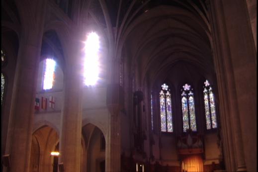
Figure 1a: (Before)
nave.hdr on an LDR display without tone mapping.
In contrast, the tone mapped image makes the colors
of the stained-glass clearly discernable (see Figure 1b). It no longer looks
like a washed-out photograph; however, we noticed exaggerated bright lights
emanating from the stained-glass windows.
We believe that this is due to the naïve histogram equalization that we
applied to the image as a part of the tone mapping algorithm, yet we did not
take into account the histogram adjustment with a linear ceiling, an
alternative approach that is described in the paper by Larson et. al [3].
The tone mapping also caused the areas inside of the
church that were not lit by natural, but artificial light to resort to warmer orange
hues. These areas have become
over-exaggerated which makes the scene appear as if were on fire. We have also lost a few details of the church
interior. For example, take a look at
the domed shaped ceiling located at the top-right of the image. The ‘before’ image (figure 1a) clearly uses
shadows and colors of brown and dark grey to imply a foreshortening
effect. The tone mapped image (see
Figure 1b), on the other hand, renders the entire section and other parts of
the ceiling with a single black color.


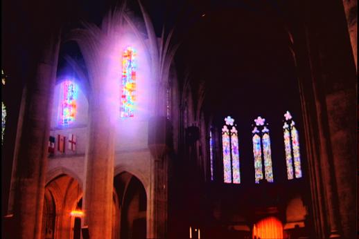
Figure 1b: (After)
nave.hdr on an LDR display after tone mapping.
Test Image
2: ‘memorial.hdr’ The
pre-tone mapped version of the next image already seems highly authentic with a
good amount of contrast in a majority of the areas, including the ceilings and
walls (see Figure 2a). The contrast
within the three stained-glass windows were the only noticeable aspects of the
image that we were hoping could be enhanced further with our algorithm.
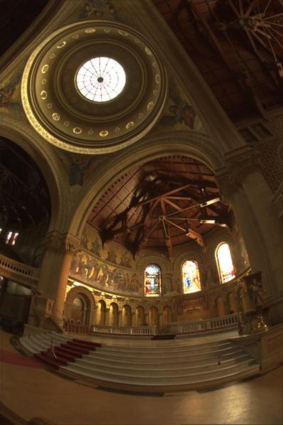
Figure 2a: (Before) memorial.hdr on an LDR
display before tone mapping.
Tone mapping definitely improved the details within the stained-glass
windows (see Figure 2b) where the depicted scene and figures in them become
discernable. Also, the dome above the
windows maintains enough of its contrast in order to remain fairly
recognizable. The church floor now seems
to be rendered more accurately due to the range in contrast, which brings out a
tiled texture compared to before where it all appeared to be of a single color.
Unfortunately, a majority of the contrast within the
interiors of the church have once again been lost. This is apparent at the top right portion of
the image where the ceiling of the church appears black. Before, a square pattern across the ceiling
was obvious, and there were reddish-brown structures that stylishly held the
top together (see Figure 2a). Also, the
colors are a lot richer, making the image appear as if a ‘dodging’ effect has
unnecessarily been applied to it.
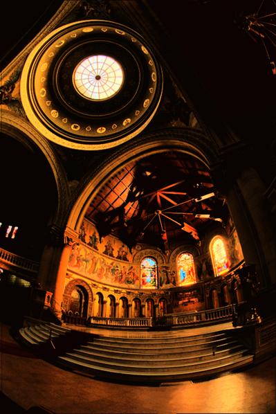
Figure 2b: (After) memorial.hdr on an LDR
display after tone mapping.
By applying a gamma correction of 2.3, we found that
we were able to retrieve some of these details back (see Figure 2c). Notice the domed ceiling located at the top
left of the image. We are now able to
see the four angels that surround the decorations around the dome. Also, the texture of the columns at the right
of the image become clearer and the range of color become more noticeable,
which was not obvious in either of the two previous images. Despite the gamma correction, there are
artifacts that remain particularly within the ceilings of the church.

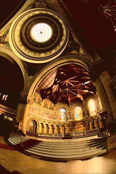
Figure 2c: (After)
memorial.hdr on an LDR display after tone mapping with a gamma correction of
2.3.
Test Image
3: ‘groveC.hdr’ The
next image is a view of the woods that looks out into the sunlight (see Figure
3a). We can see the texture of the bark
on the trees as well as the green leaves on the bushes to the left of the
image. It is obvious, however, that a
majority of the information in between the two trees to the right of the image
are lost. The extreme brightness of the
sunlight washes out any detail of the bushes that should be available to be
perceived. There appears to be a white
space, which is not an accurate representation of reality. This information would be discernable by the
human eye.

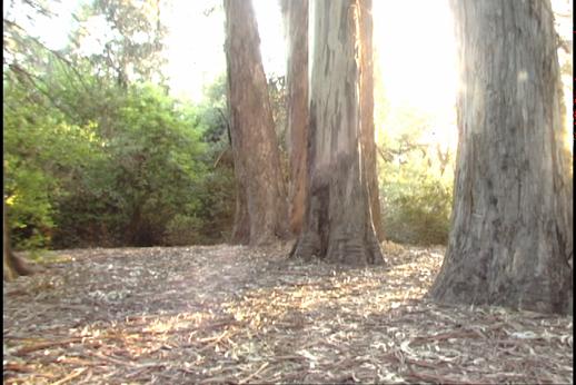
Figure 3a: (Before) grove.hdr on an LDR
display before tone mapping.
By far, the tone mapped version of
this image looks the least archaic (see Figure 3b). The most improved aspect of this image is the
sky, where the amount of contrast has been greatly enhanced. The trees in the foreground are now
complemented by the trees in the background, making the entire view a more
complete one. In addition, the texture
of the ground has gained a richer, earthier tone.
On the other hand, it is obvious
that the contrast that was present in the bushes to the left of the image as
well as the bottom portions of the trees in the foreground have become
obliterated.


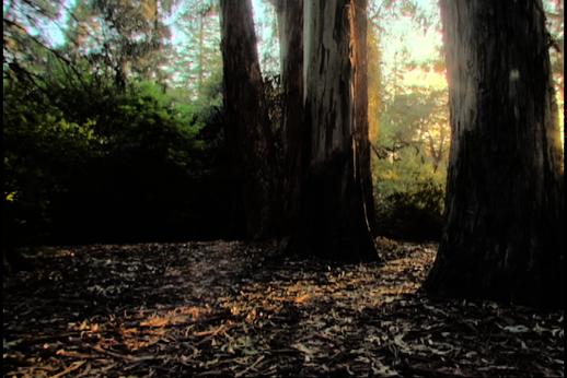
Figure 3b: (After) grove.hdr as viewed on
an LDR display after tone mapping.
With this image, we noticed that a gamma correction
at a level of 1.6 (see Figure 3c) helped brighten the really dark portions that
became evident in the image, as we just described (see Figure 3b). Fortunately, this helped gain back some of
the information that was lost. This
image also retains the information of the trees in the background as well as the
sky, but we lose a bit of the richness and contrast that we gained through our
tone mapping procedure.


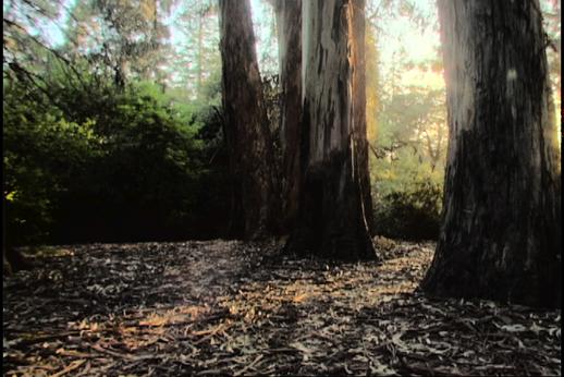
Figure 3c: (After) grove.hdr as viewed on
an LDR display after tone mapping with a gamma correction of 1.6.
Test Image
4: ‘vinesunset.hdr’ This
next image may be the most disconcerting of all the images we tested. It appears to be overlooking various houses
from a high angle against a white sky (see Figure 4a). It is almost difficult to even look into the
image, as the light from the sky is so blinding. Unfortunately as the title of the image may
suggest, this is not exactly the case.
It is actually a view of the sky as the sun is setting, which most
likely, is what the photographer was attempting to capture.
Figure 4a: (Before) vinesunset.hdr as
viewed on an LDR display before tone mapping.
We found that applying the tone mapping to this image
brings a new perspective to the original scene (see Figure 4b). It is now apparent that the sun is setting as
evidenced by the contrast within the clouds and sky. There is an orange light emanating from
behind the tree in the middle of the image, which implies that the sun is now
setting. The ‘before’ and ‘after’
examples of this image are a perfect example of how clamping effects of an LDR
display can misrepresent the artist’s intentions in a photograph or image.
The contrast along the bottom portion of the image
that makes it possible to discriminate the houses has been obliterated. The tone mapping has in a way compromised
this area in order to add contrast to the sky, which comprises a significantly
larger portion of the image.

Figure 4b: (After) vinesunset.hdr as
viewed on an LDR display after tone mapping.
Test
Image 4: ‘rosette.hdr’ Our final image is an example where our
tone mapping algorithm performs rather poorly (see Figure 5a). The interior of the church is quite
discernible, and it seems to be a rather accurate rendering of a real life
scene. It is obvious that a majority of
the artifacts that are produced are from the stained-glass window, which is
caused by the sunlight shining in.

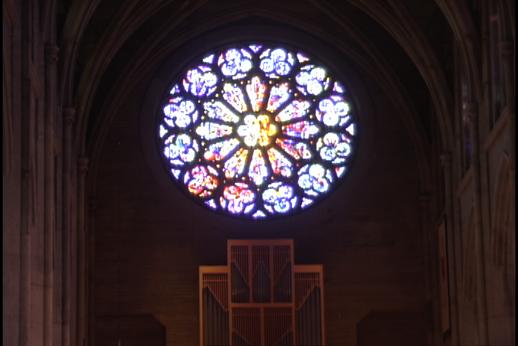
Figure 5a: (Before) rosette.hdr as viewed
on an LDR display before tone mapping.
The tone mapping adds a considerable
amount of variation to the colors in the stained-glass window, and it no longer
appears washed-out. Despite the added
variation, the window still looks overly exaggerated with glowing,
fluorescent-like lights emanating from it.
This most likely does not resemble how this window would appear in
reality.
The tone mapping also created an unnatural reddish
tinting effect around the entire room.
This glow is a bit disturbing, and by far, is not an accurate
representation of real life. This is
most likely a result of the tendency that tone mapping has to over-enhance
areas where there are relatively minor illumination variations. Compared to the other images that we tested,
the luminance values in this scene probably do not contain enough variation in
order for our algorithm to achieve a favorable effect.
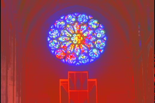
Figure 5b: (After) rosette.hdr as viewed
on an LDR display after tone mapping.
We do realize, however, that certain aspects of our
tone mapping operator would benefit from further development. Our procedure tended to exaggerate and in
some cases darkened, or degraded other areas that were not originally affected
by the clamping effects of the LDR display device (e.g. room interiors). These areas already contained a considerable
amount of contrast mainly due to the fact that the illumination levels of these
areas were not located at the extreme ends of the luminance scale. The tone mapping process often reduced
luminance resolution in areas of small variation in order to handle the
extremes in luminosity of the original image.
Our algorithm demonstrated a significant improvement
within various areas of scenes lit by natural light (e.g. stained-glass
windows, areas looking out into natural light).
These sections are the areas most affected by clamping, because their
illumination levels occur at points that are too high to be rendered accurately
with low dynamic range devices. The tone
mapping acknowledges this and gives consideration to the areas with extreme
levels of luminosity.
Conclusions
Advancements in the computer and its technologies
have come a long way. There will be a
continual demand for researchers to invent faster processors that outperform
last year’s models or video game professionals to release newer versions of
games that exceed the standards of graphics that we see today. Yet in order to keep up with the latest
technologies, it is important that the high expectations we place on our
computer hardware and peripherals parallel those that are used to enhance the
visual experiences that accompany these developments. After all, who wants to take a family reunion
picture outside on a sunny day with an advanced digital camera only to find
that viewing it on the home computer makes everyone appear either faint or
washed-out?
It is not to say that all of the
problems with computer technology may be solved with improvements in the
reliability and fidelity of output devices.
Just by trading in your LDR monitor for an advanced one that has the
ability to display HDR, the visual experience you encounter through viewing
your monitor may not necessarily be a replica of real-life. There are many more things that will have to
be discussed in order to render a real-life scene with high fidelity. This
depends on the subjective nature of the human visual system (HVS), which is a
difficult thing to model mathematically.
There are many complexities within the HVS that are either poorly
understood or too complex for scientists to completely capture.
For example, humans have an ability known as
peripheral vision. It includes a field
of view that is comprised of not just what is directly in front of you, but
also seeing what is a little to the left and right of you. This “subjective experience” is something
that goes a bit beyond a simple, ordinary computer monitor or photographed
image; however accurate brightness or luminance of a scene can go a long way in
extending subjective performance.
Our algorithm improved the extremely bright areas
that resulted from intense illumination and appeared washed out, but as a
trade-off it suffered from a degradation of luminous acuity in areas of subtle
variation. In other words, it does the
exact opposite of what many LDR display devices do, which is to correctly
display areas that are not of extreme brightness or darkness, but inaccurately
represent areas that do not fall into this category.
Overall, we feel that our algorithm properly
demonstrated our idea. Often times, a
significant portion of data in an image may be lost or indiscernible to the
viewer using a low dynamic range display.
Concerning images with little contrast, this problem may seem trivial,
yet it is a serious issue that affects images containing high contrast
elements. Essential details that are
crucial to the various elements of an image may be misrepresented, detracting
from the overall meaning of the image.
Luckily, there is a solution to this mapping
problem. It has been a heavily studied
topic, and collaborative efforts are being made by accomplished researchers to
find alternative methods. It may be
years before a perfect tone mapping operator is found, but it is comforting to know
that the research has come a long way.
REFERENCES
[1] Ferwada,
James A. Elements of Early Vision for Computer Graphics. IEEE Computer Graphics and Applications 21.5 (2001): 22-33.
[2] Larson,
Gregory W. Radiance: Synthetic Imaging
System. The
28
Sept. 2005 <http://radsite.lbl.gov/radiance/>.
[3] Larson,
Gregory W., Holly Rushmeier, and Christine Piatko. “A
Visibility Matching Tone Reproduction Operator for
[4] HDR
Shop. USC Institute of Creative
Technologies. 11 Aug. 2005 <http://gl.ict.usc.edu/HDRShop/>.
[5] Hearn,
Donald and M. Pauline Baker. Computer Graphics with OpenGL.
[6] Meyer,
Jon. “The Future of Digital Imaging –
[7] Spencer,
Greg, Peter Shirley, Kurt Zimmerman, and Donald P. Greenberg. “Physically-Based
Glare Effects for Digital Images.” Proceedings of the 22nd annual conference on
Computer graphics and interactive techniques 520 (1995): 325-334.