Abstract
This paper describes the design and animation of a new data structure called a Kinetic PR Quadtree. The impetus for this project was the desire to grant the traditional PR quadtree the ability to hold non-stationary data points with velocity vectors in finite, 2-dimensional space. The movement of the data points over time would change the structure of the PR quadtrees subtrees. The main focus of the project was implementing this ability for the PR quadtree and animating the changes in quadtree structure during the data points movement.
Introduction
Designing efficient data structures has always been an important field in computer science. An interesting set of data structures are the kinetic data structures. These objects do not simply hold static data or changing data, but data that, as it undergoes change, also changes the form of the structure that contains it.
Kinetic data structures are often spatial data structures. If a data structure represents an objects shape and location in space, and the object is transforming, then the data structure should transform to accommodate it. Li Zhang, a Ph.D. student at Stanford University, has researched this area, dealing with proximity between objects, collisions of objects, and the visibility of objects. At their most basic levels, these studies involve moving and deforming objects. Such activity is performed using what is called the kinetic data structure framework, which was proposed in 1997. In regard to objects under this framework, Zhang writes, "a geometric structure is maintained in an event driven manner where the structure is certified by a set of primitive conditions and examined only at the times when one of the conditions fails; or in other words, a geometric structure is maintained by animating a proof of correctness over time."
The data structure in this project does not deal with the representation of a small number of complex objects interacting and moving in space, but the representation of a large number of simple objects moving in space. As objects change their position, the data structure transforms, which is the case with kinetic data structures. There are similarities to the aforementioned framework in the form of rules obeyed by the structure whereby if a rule is violated, the structure changes.
Introduction to the Kinetic PR Quadtree
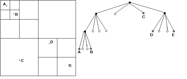
The Kinetic PR Quadtree derives its name from the PR quadtree (Samet 87-95) and the fact that it contains kinetic data, that is, data that can move. The Kinetic PR Quadtree stores data points, or points, in a 4-ary trie structure. The quadtree divides the data points such that each cell, a square division of finite space also called a quadrant, contains at most n points, where n is a user-defined size from 1 to 5. A function with the parameters time, velocity of a point, and initial position of a point determines a points position. Points with non-zero velocity change their position over time, eventually intersecting the boundaries of their cells. A priority queue stores these intersections, ordering them such that the intersection that will happen soonest is accessed first. The Kinetic PR Quadtree changes its structure based on the order of these intersections. Figures 1 through 6 show a simple visual example of the structure in action.
Figure 1____________________________Figure 2_______________________________________

Figure 1 is the spatial representation of a Kinetic PR Quadtrees initial state where the bucket size is 1. It contains five data points, labeled A to E. Black lines show the cell boundaries. The gray dots represent the data points. Figure 2 shows the tree representation. Black circles are non-leaf nodes. White circles are empty leaf nodes. Gray circles are leaf nodes containing the labeled data points. Though not displayed, the vectors for the data points are as follows: A is moving to the right, B is moving to the right, C is moving down and right, D is moving to the left, and E is moving to the left. A is moving somewhat slower than B, and E is moving slower than D.
Figure 3___________________________Figure 4_____________________________________
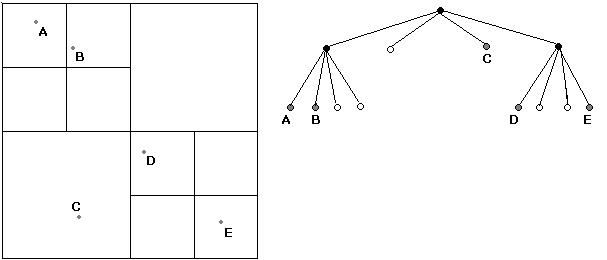
Figures 3 and 4 represent the previous Kinetic PR Quadtree at time equals 5. As B moved out of its cell, one of the divisions separating A and B disappeared because of a rule violation. This rule is that if a divided cell must contain more than the maximum to justify the division. (The maximum in this case is 1.) Because the divided cell once containing A and B now holds only one point, its division was removed to make its four quadrants into one larger, undivided cell.
Figure 5____________________________Figure 6____________________________________
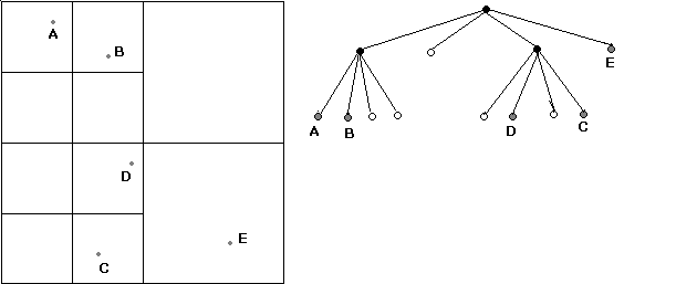
Figures 5 and 6 represent the previous Kinetic PR Quadtree at time equals 10. D and E experience a similar situation. As D moved into a cell containing C, a new division materialized to accommodate the two data points out of another rule. A cell that contains more than the maximum allowed number of points must be divided until the new cells created in the division each hold no more than the maximum allowed points or are divided as well.
Three main parts comprise the Kinetic PR Quadtree: the data points, the PR quadtree, and the priority queue.
Definition and Description of Parts and Their Functions
Data Points (Points). Data points contain the user-input information. The data points exist as dimensionless points in 2-dimensional space, but appear as small circles for visibilitys sake in the animation. Each data point must have three fields: NAME, STPT, and VEC. The NAME field is a string of characters that represents the name of the data point. The STPT field contains the x and y coordinates of the data points position when time equals 0. The VEC field contains the data points velocity vector in the x and y directions. Using the STPT and VEC fields and the current time, the movement function in shown in the algorithms can find the current position of the data point. For convenience sake, two fields called X and Y were also used to hold the current position of a data point so that the program only has to call the function once when the current position is referenced more than once.
Data points are stored in the leaf nodes of the PR quadtree. Leaf nodes can hold up to n data points. The data points will eventually strike the cell walls, also called boundaries. The calculated intersections of the points with the cell walls of the PR quadtree are placed in the priority queue.
PR Quadtree. The PR quadtree is a 4-ary trie that associates data points with quadrants. The P in its name stands for "point" and the R stands for "region" (Samet 87). The region of the tree is a finite 2-dimensional square. Because it is a trie, the PR quadtree stores the data points at its leaf nodes. The necessary fields for the quadtree are the priority queue (UPDATES) and ROOT.
The ROOT field is a data node. Each data node must contain seven fields: NW, NE, SW, SE, NODETYPE, VS, and SQ. SQ contains the dimensions of the quadrant the data node represents in terms of the quadrants center and the length of one of its sides. NODETYPE determines the type of the node. If NODETYPE is -1, then the data node is empty. If NODETYPE is 0, then the data node is a non-leaf node. If NODETYPE is 1, then the data node is a leaf node containing a data point. NW, NE, SW, and SE are the children of the data nodes and are all data nodes themselves if NODETYPE is 0. Otherwise they are all null. The VS field is the n data points contained by the node if NODETYPE is 1. Otherwise it is null.
The function of the PR quadtree is to contain the data over a finite plane. The PR quadtrees function is constrained by two rules:
Priority Queue. The priority queue in the Kinetic PR Quadtree is a heap that sorts by time value, i.e., the first element taken from the heap is the one that will intersect with a boundary first. Sorting by time allows the PR quadtree to change its shape in chronological order. The priority queue is a field of the PR quadtree and is accessed as time advances.
The individual elements of the priority queue have five fields: TARGET, V, TIME, INTERSECTION and VERSION#. TARGET is a link to the data node currently containing the data point of interest. V is a copy of the data point. TIME is a real number set to the time of intersection. INTERSECTION is the coordinates of the intersection of the moving point and the boundary. VERSION# is an integer that determines whether the element is still valid. The priority queue has a complementary hash table that stores up-to-date version numbers for each data point. If the version number in the hash table entry for a particular element does not match the version number in the priority queue element, then the element is obsolete and disregarded. The updating of version numbers is essential because divisions both appear and disappear as the tree changes, causing a points next intersection to change, too.
Summary, Interrelation of Parts, and Basic Internal Operation Description
The Kinetic PR Quadtree does the following when dealing with points moving over time. While time is 0, the data points are inserted, and the priority queue intersection values are initialized. Time will increment steadily, and the priority queue will continue to dequeue intersections as they occur. For each valid intersection, the point will be removed from its old cell and reinserted into its new cell in the PR quadtree. Divisions are created and removed as necessary. The priority queue is updated during this process if the subsequent intersections of points change. This process continues infinitely or until some time limit is reached.
The three major parts of the Kinetic PR Quadtree work together both to hold input information and allow movement over a period of time, while staying within the rules of a PR Quadtree.
In an operating cycle, the user first inputs all the points before time begins to increment. This information includes NAME, STPT, and VEC for each point. The points enter the PR quadtree, which creates divisions as needed. The priority queue also initializes an intersection for each addition, calculating the first boundary to be struck by each point.
The Kinetic PR Quadtree has an animation implementation. In order to generate smooth animation, the program sends the quadtree the time updates, incrementing at a constant, user-defined rate. The program iteratively sets the time to higher and higher values infinitely or until the program reaches a user-defined time limit.
At each iteration, the priority queue dequeues every element with a time less than or equal to the current time sent into the PR quadtree. For each of these elements, the following is performed. The version of the element is compared against the value in the hash table. If they do not match, then the elements intersection is not valid, and the program disregards it. Otherwise, the program continues by checking to see if the intersected boundary is one of the outer walls of the PR quadtree. If so, then the point must bounce because it can not exit the range. Bouncing is achieved by changing the sign of the appropriate direction vector and altering the initial position. If the point does not hit an outer wall, the program skips this step. The algorithm for bouncing is shown later.
The point is removed from the PR quadtree. The program then reinserts the point. A reinserted point is always positioned on a line between quadrants. The PR quadtree reinserts the point in the correct node, and thus correct quadrant, by viewing the velocity vector of the point. The point ends up in whichever quadrant is in the vectors direction. The other important phase of reinsertion is the creation of new divisions as necessary. If the quadrant already contained n points, then divisions occur until the n+1 points end up in cells each containing n or less data points. This is accomplished by replacing the leaf node containing the present point with a non-leaf node. The children of this node are all leaves, and the present point and entering point enter the nodes that represent their spatial positions. If the n+1 points end up in the same node, this process repeats itself on that leaf node until they end up in separate leaf nodes. The final phase of reinsertion is the addition of elements to the priority queue. If the point entered an empty quadrant, an element based on its next calculated intersection is added to the priority queue and the version number is incremented for both that element and the hash table. Otherwise, the program performs the same procedure for both the entering point and the points already present in the quadrant. The algorithm that updates the version appears later.
The PR quadtree then removes divisions that violate its rules. From the ROOT node, the PR quadtree travels down via the child links to the cell the intersecting point left. From there it recurses back to the parent node, checking all the children. In this process, if the program finds there are less than n+1 points in a divided space, the program eliminates the division. This means that a non-leaf node with four leaf children is replaced with a non-empty leaf node. This leaf node contains the points present among the four children of the original non-leaf node. This process repeats on all parents back up to the ROOT. If divisions are removed, the affected points versions are updated on the hash table, and a new intersection is calculated and added as an element to the priority queue for each of them.
After all the intersections that occur before the current time are dequeued and run through this procedure, a frame of animation depicting the updated PR quadtree appears on the screen. If the time limit has not been reached, the entire process repeats itself and subsequent frames of animation appear on the screen, displaying the PR quadtrees movement over time.
Algorithms
The two most significant processes in the rearrangement of the Kinetic PR Quadtree structure are the reinsertion of points and removal of points that occur inside the function labeled setTime, which updates the tree to the time given in a parameter. Other important algorithms included are the ones for Bounce, getPos, and the general algorithm for updating the priority queue and hash table.
setTime
//This function updates the tree to the appropriate time
setTime ( time, i
ValidEntry ßfalse
q1=dequeue(UPDATES)
if the VERSION entry for q1s name matches q1s version number
then
ValidEntry ßtrue
if the point in q1 intersects an outer wall
of the PR quadtree then
pnode ß
TargetOf(q1)
v1 ß
Vertex(q1)
v1 ß
Bounce(v1)
deleteVertex(pnode,v1)
if (Size(pnode) ==
0) then
Bucket(pnode) ß null
NodeType(pnode) ß -1
Reinsert( ROOT, v1, getTime(q1),
pointOfIntersection(q1) )
RemoveDiv( ROOT, Xcenter(pnode),
Ycenter(pnode), getTime(q1) )
else
pnode ß
TargetOf(q1)
v1 ß
Vertex(q1)
deleteVertex(pnode,v1)
if (Size(pnode) ==
0) then
Bucket(pnode) ß null
NodeType(pnode) ß -1
Reinsert( ROOT, v1, getTime(q1),
pointOfIntersection(q1) )
RemoveDiv( ROOT, Xcenter(pnode),
Ycenter(pnode), getTime(q1) )
else Information is outdated, so no action is needed.
return ValidEntry
_____________________________________________________________
Reinsert
//This procedure reinserts a point into the correct position of the
PR quadtree
Reinsert ( current, pt, time, spot)
//current is the current node
//spot is the location of the point
//pt is the data point (data point is also called vertex in this context)
flag ß false
if (NodeType(current) == 0) then // We are at a nonleaf
node
Recurse downward through the tree. Compare the x
and y values of spot to current so:
if (X(spot) < Xcenter(current)) and
(Y(spot) < Ycenter(current)) then recurse to SW
if (X(spot) Xcenter(current)) and
(Y(spot) < Ycenter(current)) then recurse to SE
if (X(spot) < Xcenter(current)) and
(Y(spot) Ycenter(current)) then recurse to NW
if (X(spot) Xcenter(current)) and
(Y(spot) Ycenter(current)) then recurse to NE
In the cases where an x or y value of spot is equal
to an x or y value of current,
then recurse in the quadrant in the direction in
which the VelocityVector(pt) is pointing.
In the special case when the child in the recursing
direction is null, do the following:
flag ßtrue
quad ß
recursing direction (either NE, NW, SE, or SW)
if (flag) then
P ß
new PrNode that holds pt in its bucket with center
and length corresponding to the quad child of current
NodeType(P) ß
1
SON(current,quad) ß
P
Update VERSION and UPDATES
for pt
else // we are at a leaf node (either empty, full, or non-empty/non-full)
if (NodeType(current) == -1) then
Add( Bucket(current), pt)
NodeType(current) ß
1
Update VERSION and UPDATES
for Bucket(current)
else if (NodeType(current) == 1) then
if (Size(current)
< bucketSize) then //not full
Calculate current positions for all points in Bucket(current) using getPos
Add( Bucket(current), pt)
Update VERSION and UPDATES for Bucket(current)
else //full so we
split
pts ß Bucket(current)
Bucket(current) ßnull
NodeType(current) ß 0
Calculate current positions for all points in pts using getPos
keepSplitting ß true
X ß Xcenter(current)
Y ß Ycenter(current)
LX ß Length(current)
LY ß Length(current)
curr2 ß current
while
(keepSplitting) do
s1 ß quadrant of curr2 where we find
pt
Xtemp ß X
Ytemp ß Y
X ß X+XF(s1) * LX //XF returns .25
for E and -.25 for W
LX ß LX/2.0
Y ß Y+YF(s1)*LY //YF returns .25 for
N and -.25 for S
LY ß LY/2.0
k ß 0
while (k < Size(pts)) do
UQ ß quadrant of curr2 where we find
pts(k)
if SON(curr2,UQ) is null or has NodeType of 1 then
P ß new PrNode that holds pts(k) in
its bucket with center and length of the UQ child of
curr2 NodeType(P) ß 1
SON(curr2,UQ) ß P
Update VERSION and UPDATES for pts(k)
else // there is between 1 and bucketsize-1 points present
Add( Bucket(SON(curr2,UQ)), pts(k))
Update VERSION and UPDATES for pts(k)
k++
if ((SON(curr2,s1) == null) or (NodeType(SON(curr2,s1))
== -1) or (size(SON(curr2,s1)) < bucketSize)) then
keepSplitting ß false
else
keepSplitting ß true
pts ß Bucket(SON(curr2,s1))
curr2 ß SON(curr2,s1)
NodeType(curr2) ß 0
Bucket(curr2) ß null
// out of while loop
// should be able to add pt to SON(curr2,s1)
if ( (SON(curr2,s1) == null) or (NodeType(SON(curr2,s1))
== -1) ) then
P ß new PrNode that holds pt in its
bucket with center and length of the UQ child of curr2
NodeType(P) ß 1
SON(curr2,UQ) ß P
Update VERSION and UPDATES for pt
else // there are already points, but we can add the latest one
Add( Bucket(SON(curr2,UQ)), pt)
Update VERSION and UPDATES for Bucket(SON(curr2,UQ))
else ERROR: NodeType not 1, 1 or 0
___________________________________________________________________________
RemoveDiv
// This function removes superfluous divisions from the PR quadtree
(divisions that hold less
// than the bucketsize+1 of data points
RemoveDiv ( current, x, y, time )
if ( (current == null) or (NodeType(current) == -1) or
(NodeType(current) == 1) ) then
return false
else
stable ß false
if (Xcenter(current) x) then
if (Ycenter(current)
y) then
stable ß RemoveDiv ( SON(current,SW),x,y,time)
else stable ß
RemoveDiv ( SON(current,NW),x,y,time)
else if (Ycenter(current) y)
stable ß RemoveDiv( SON(current,SE),x,y,time)
else stable ß
RemoveDiv( SON(current,NE),x,y,time)
j ß 0
counter ß 0
temp ß null
if (not(stable)) then
if (SON(current,
NW)!=null) then
if (NodeType(current, NW)==0) then
counter+=bucketSize+1
else if (NodeType(current,NW))==1) then
counter += Size(SON(current, NW))
Add( temp, data points in SON(current, NW))
if (SON(current,
NE)!=null) then
if (NodeType(current, NE)==0) then
counter+=bucketSize+1
else if (NodeType(current,NE) ==1) then
counter += Size(SON(current, NE))
Add( temp, data points in SON(current, NE))
if (SON(current,
SW)!=null) then
if (NodeType(current, SW)==0) then
counter+=bucketSize+1
else if (NodeType(current,SW)==1) then
counter += Size(SON(current, SW))
Add( temp, data points in SON(current, SW))
if (SON(current,
SE)!=null) then
if (NodeType(current, SE)==0) then
counter+=bucketSize+1
else if (NodeType(current,SE)==1) then
counter += Size(SON(current, SE))
Add( temp, data points in SON(current, SE))
if (counter=(bucketSize+1))
then
//No more removal of splitting needed
stable ß true
else // We must remove
the division because we have insufficient points
if ((temp == null) or (Size(temp) == 0)) then
NodeType(current) ß -1
Bucket(current) ßnull
else // This means there is a vertex so the NodeType must be 1
NodeType(current) ß 1
Bucket(current) ß temp
SON(current,NW) ßnull
SON(current,NE) ßnull
SON(current,SW) ßnull
SON(current,SE) ßnull
stable ß false
Calculate current positions for all points in Bucket(current) using getPos
Update VERSION and UPDATES for Bucket(current)
return stable
____________________________________________________________________________________
Algorithm for Computing Next Intersections and Updating Versions
//This algorithm is basically the same when used in different cases
in Reinsert and RemoveDiv.
//It was taken out simply to avoid having it written over and over
and increasing the document
//length. In the cases where we only update one point, you can simply
do the process within the //while loop just once.
//current is a data node
//VERSION is the hash table
//UPDATES is the priority queue
//getCollisionTime(
) calculates the time of the next collision
//isZero finds whether a vector value is zero
//SetIntersection(
) sets the intersection for the data point dealt
with
//GetIntersection(
) gets the intersection for the data point dealt
with
j ß 0
while (j < Size( Bucket(current)))
i ß GetNumber(VERSION,
GetElement(current, j))
PutNumber(VERSION, GetElement( current, j), i+1))
if (NOT( isZero( VEC( GetVertex( current,
j)))))
//This previous line removes the cases where the
point is not moving, which can cause
//an infinite loop (if a motionless point lies on
a line it is forever intersecting it).
q1 ß
new QNode( time, GetCollisionTime( SQ(current), GetVertex(current, j) ),
i+1, GetVertex(current, j), current)
HIT ß
GetIntersection(SQ(current), GetVertex(current, j) )
SetIntersection(q1, HIT)
enqueue(UPDATES, q1)
j ß j+1
_____________________________________________________________________________________
getPos
// This function finds the current position of a point in space based
on its initial position, its
// vector and time
getPos ( start, vector, time )
// start is the initial position of the data point in 2-dimensional
space
// vector is the vector of the data point in 2-dimensional space
// vector represents the distance moved in 2-dimensional space for
every 1 unit of time
// time is the current time along the vector from the given initial
position
p ß start + vector * time
return p
_____________________________________________________________________________________
Bounce
// This function takes a vertex of a data point (which contains the
information about initial
// position and vector). It flips these values based on which wall
is struck by the data point.
// V has X and Y values too. These were set to the position of intersection
when the data point
// was added to the priority queue.
Bounce ( V )
Start ß STPT(V)
Vec ß VEC(V)
if (X(V) == theMax) // V has hit the extreme right wall
STPT(V) ß new
point( theMax*2.0 X(Start), Y(Start))
VEC(V) ß new
point(-X(Vec), Y(Vec))
Vec ß copy of
VEC(V)
Start ß copy
of STPT(V)
if (X(V) == theMin) { // V has hit the extreme left wall
STPT(V) ß new
point( theMin X(Start), Y(Start))
VEC(V) ß new
point(-X(Vec), Y(Vec))
Vec ß copy of
VEC(V)
Start ß copy
of STPT(V)
if (Y(V) == theMax) { // V has hit the extreme top
STPT(V) ß new
point( X(Start), theMax*2.0 Y(Start))
VEC(V) ß new
point(X(Vec), -Y(Vec))
Vec ß copy of
VEC(V)
Start ß copy
of STPT(V)
if (Y(V) == theMin) { // V has hit the extreme bottom
STPT(V) ß new
point( X(Start), theMin Y(Start))
VEC(V) ß new
point(X(Vec), -Y(Vec))
Vec ß copy of
VEC(V)
Start ß copy
of STPT(V)
return V
______________________________________________________________________________________
User Operation and Animation of the Kinetic PR Quadtree
You can reach the java applet for the animation at test0.htm
Before inputting the data points the user sets the bucket size for the Kinetic PR Quadtree cells. Before time starts incrementing, the user inputs the data points. This is done by clicking the mouse on the 2-dimensional representation of the Kinetic PR Quadtree in the Java applet to indicate the initial coordinates and dragging to indicate the vector of the point corresponding to distance and direction moved in one time unit. It receives a default name. For data points with more accurate initial positions and vectors, the user can input a name and real numbers for the x and y coordinates of the starting position and vector in the appropriate fields. After inputting information for a specific point, the user selects the "make point" button to create the point. Before starting the animation, the user can also enter a time for the program to terminate its animation. Once the animation begins, the user controls the length of pauses between successive frames of animation, and the user can manipulate how fast time increments. The animation displays the moving 2-dimensional space as shown in Figures 1, 3, 5 and on the following pages.
Future Study
The most obvious avenue of research following the creation of the Kinetic PR Quadtree are tests of the efficiency of the data structure and the algorithms that update the quadtree with regard to saving time and space. A data structure that might be used for such a comparison is a grid that contains mobile data points but has set cell divisions and buckets of infinite capacity (for the cases where all the points converge in one area for some reason). I would speculate at this point that for large data that is randomly distributed over the planar range of the data structure, the Kinetic PR Quadtree would be more efficient.
Allowing points to move in a more interesting manner than straight-line vectors bouncing off the walls would be another interesting feature. The possibility currently being investigated is applying a force of gravity to the points that makes them gradually fall to the bottom of the screen. Another possibility is giving points some knowledge about their whereabouts in space and the locations of other points. With this model, we could create points that might attract or repel one another, perhaps even mimicking herd-like or solitary behavior of animals in a wilderness environment at some point. The same basic algorithms for the Kinetic PR Quadtree and the triad of data points, quadtree and priority queue, should retain their basic attributes.
Frames of Animation Example 1: Explosion from the center in a 256 x 256 square with cell capacity of 3.
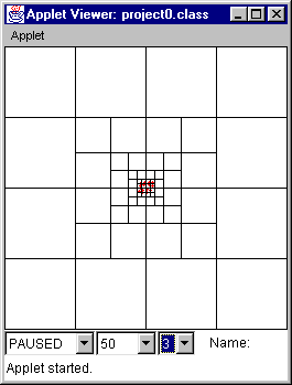
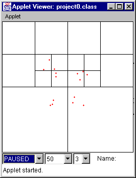
Figure 7 Figure 8
Figure 7 Initial state: all points clustered at the center, with velocity vectors directed outward.
Figure 8 At time = 5, the points spread. The number of divisions decreases as distribution becomes more uniform.
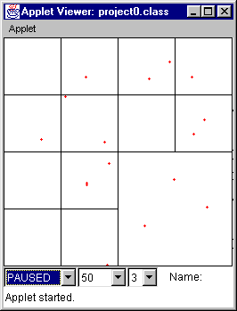
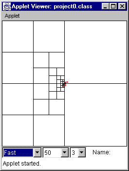
Figure 9 Figure 10
Figure 9 At time = 48, the points have been bouncing off the walls and are more uniformly distributed.
Figure 10 At time = 256, the points have all returned to the center of the space. This is due to the fact that regardless of the velocity vectors, the points have moved distances bound by a range of 256 in x and y directions. If points start clustered they tend to "recluster" at times that are multiples of the bounds.
Example 2: Here is a series of more complex
random examples on a field of 512 x 512 pixels (cell capacity of 3).
(This looks better with Netscape Navigator.)
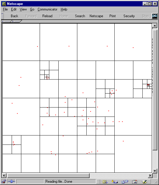
Figure 11 (time = 0)
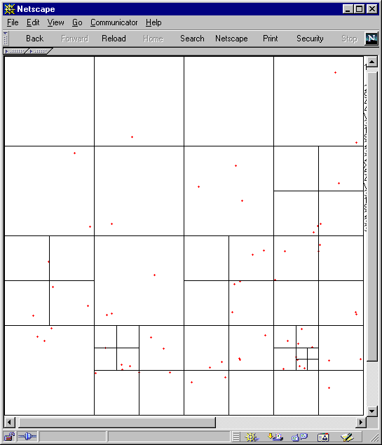
Figure 12 (time = 10)
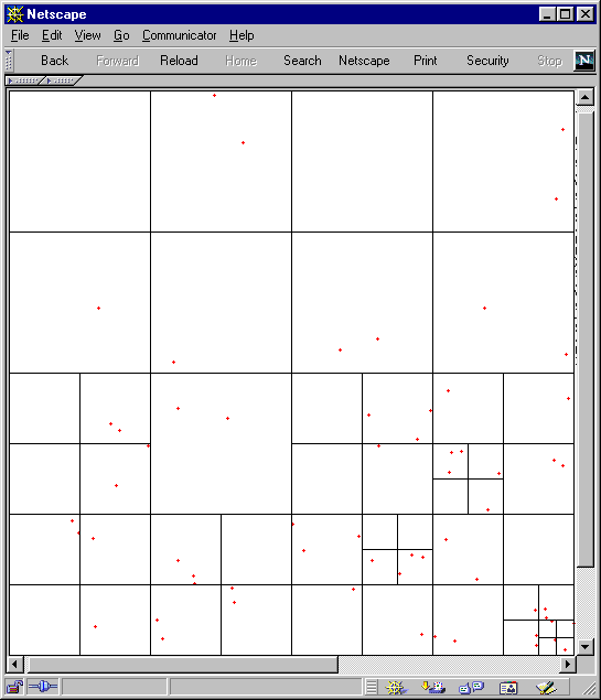
Figure 13 (time = 20)
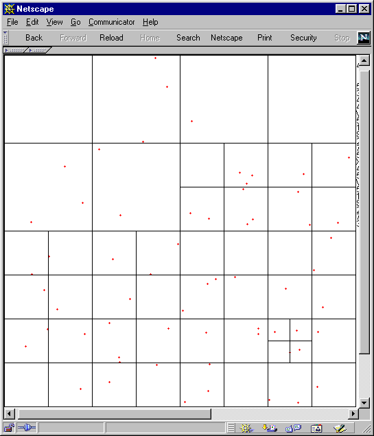
Figure 14 (time = 40)
Again we can see from Figure 11 14 that the distribution becomes fairly even under random circumstances over time and the number of cells dividing the points decreases.
Example 3: A series of smaller "explosions" at different areas on the range (256 x 256) with cell capacity of 2.
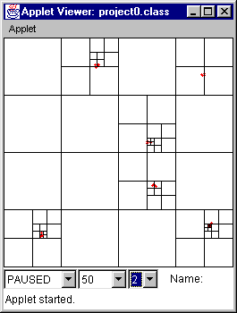
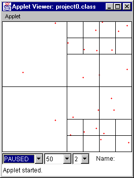
Figure 15 (time = 0) Figure 16 (time = 32)
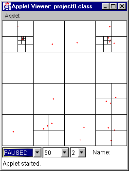
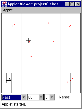
Figure 17 (time = 128) Figure 18 (time = 256)
Figure 15 Initial state.
Figure 16 Typical picture of animation, where points are fairly evenly distributed.
Figure 17 At time = 128, some of the points "recluster."
Figure 18 At time = 256, some of the points "recluster" again. There is not a widespread "reclustering" of all the points because they did not all start at a position which was relatively equally distant from all walls.
Thanks
I would like to thank the people for their help on this project:
Winder, Ransom. Examples of a Point-Region Quadtree with moving points
or a "Dynamic PR Quadtree". 29 September 2000.
<http://users.starpower.net/rwinder>.
Zhang, Li. Lis Research Page. Computer Graphics at Stanford
University. 23 November 2000.
<http://graphics.stanford.edu/~lizhang/research/>.