


We have by now assembled enough ideas to be able to give a more thorough statement of the rules of elementary quantum mechanics.
A. At any moment, a given physical system S is in some state, which is
(described by) a wavefunction  .
.
B. This state can change over time, since it is a function of time, as well as of position.
C. Normally this change over time is a well-defined and predictable
evolution given by the time-dependent Schrodinger equation (TDSE).
We will not describe this equation in detail, except to say that it
specifies exactly how changes under ``normal'' conditions, ie,
when the system is not being subjected to a measurement.
D. However measurement in general tends to cause the system to change
suddenly and unpredictably from whatever state it was in to
a new state
 , such that
satisfies TISE
(ie, is an eigenfunction or eigenstate) for the operator
, such that
satisfies TISE
(ie, is an eigenfunction or eigenstate) for the operator  corresponding to the observed quantity
  ; and observed value
  of is the corresponding eigenvalue.
E. If already is an eigenfunction of then there is no
change at all resulting from the measurement, ie the system stays
in state .
F. But if is not an eigenfunction for the quantity
being measured, then the state will definitely change into one of
the eigenfunctions  of . But which one it changes into
(and therefore which eigenvalue is observed) is not determined
but is rather a matter of chance (probabilities).
of . But which one it changes into
(and therefore which eigenvalue is observed) is not determined
but is rather a matter of chance (probabilities).
G. The probability that changes to a particular eigenstate, say
 , can be computed very precisely
as follows. We write as a ``superposition'' (linear
combination) of all the eigenstates of :
, can be computed very precisely
as follows. We write as a ``superposition'' (linear
combination) of all the eigenstates of :

where the sum can be infinite (and may even in some cases need to
be written as an integral instead). This is the ``superposition
principle'', namely that for any observable the eigenstates
form a ``complete'' set so that any wavefunction at all can be
written uniquely as such a linear combination (or weighted sum) of
them. And now the probability that a given is the one
changes into is simply  . Absolute values are needed since
the coefficients
. Absolute values are needed since
the coefficients  are allowed to be (and in general need to
be) complex numbers.
are allowed to be (and in general need to
be) complex numbers.
The coefficients can be thought of as weights indicating how
strongly each is part of , or to what extent has value
 , althought the precise meaning is in terms of the absolute value
squared.
, althought the precise meaning is in terms of the absolute value
squared.
Thus a particular state that a system S might be in at some time t, might have more than one "value" of some variable (such as momentum) at that time. This is so even if the system is a single particle. People sometimes speak as if the particle had many "incarnations" all at once, or parallel existences. But this also means that we cannot ``see'' (measure) these values, until we set up a measuring apparatus which collapses that superposition state into just one and the rest disappear. It is as if we were to say ``there is an orange and purple hippopotamus in this room whenever no one is there to see it.'' And yet, although we never observe the superposed states, although all but one disappears when we try to observe the given property, the math works out in perfect agreement with experiment! Nature seems to require that the superposed states be there, in order to interfere with each other in a wavelike manner, so that when they collapse into just one observed state and value, the results when averaged over many cases give the wavelike pattern that we find experimentally.
At last we are done with our exposition of elementary quantum mechanics. We will apply it, below, to the polarization experiment in order to get a feel for how it works.
But we have already seen the essential ingredients for quantum computation, namely that (i) a system may be in a state that does not have a well-defined value for some observable quantity; but (ii) that state will change into a new state that does have such a value if we try to observe that quantity; and (iii) that in a sense the old state has all possible values of that observable implicitly represented as a superposition of all the eigenstates for that quantity; and finally (iv) until we perform that measurement, the system will evolve predictably (and therefore with all the implicit eigenstates evolving along with it).
To end our discussion, we briefly present two standard applications of quantum mechanics. Note well: these are not examples of quantum computation!
The first one is a quantum mechanical description of the polarization
phenomenon. A given photon at any time is in a state  which may
or may not be a vertical-filter eigenstate, ie it may or may not
already be vertically polarized. But if not, then it is a
superposition of eigenstates, of which there turn out to be exactly
two key ones: vertical and horizontal. That is, observing the photon
with a vertical filter means finding out whether it passes through
(this vertical state we write as
which may
or may not be a vertical-filter eigenstate, ie it may or may not
already be vertically polarized. But if not, then it is a
superposition of eigenstates, of which there turn out to be exactly
two key ones: vertical and horizontal. That is, observing the photon
with a vertical filter means finding out whether it passes through
(this vertical state we write as  ) or not (the horizontal state,
written
) or not (the horizontal state,
written  ). Any weighted sum
 of these represents a
superposed state in which the photon has a mix of the vertical and
horizontal states (as long as it is normalized so that the total
probability is right:
of these represents a
superposed state in which the photon has a mix of the vertical and
horizontal states (as long as it is normalized so that the total
probability is right:
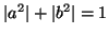 ). The verticality operator
 in this case simply operates on this superposed state and
returns the part only. Thus itself is an eigenstate (with
eigenvalue 1, meaning ``yes'') and so is with eigenvalue 0
(``no''). Now what about a 45-degree polarization? A photon
in that state has a perfectly even mix (superposition) of the
vertical and horizontal:
in this case simply operates on this superposed state and
returns the part only. Thus itself is an eigenstate (with
eigenvalue 1, meaning ``yes'') and so is with eigenvalue 0
(``no''). Now what about a 45-degree polarization? A photon
in that state has a perfectly even mix (superposition) of the
vertical and horizontal:
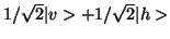 . And the
probability a photon in this initial state collapses into state
(when we measure it with a vertical filter) we can compute: it is just
the absolute value squared of the coefficient of in that
superposition, namely
. And the
probability a photon in this initial state collapses into state
(when we measure it with a vertical filter) we can compute: it is just
the absolute value squared of the coefficient of in that
superposition, namely
 .
.
Our second application concerns chemistry, or more specifically the energy levels of electrons in an atom (which determine the chemical properties of that element). An electron in an atom is in a so-called bound state: it cannot move feely but rather is constrained to stay fairly near the nucleus by the attractive electrical force between it and the protons in the nucleus. One can write a version of TISE for the energy observable, and solve it for the various energy eigenfunctions and associated energy eigenvalues. It turns out that the mathematics gets very tricky, and so people make simplifying assumptions in order to get approximate solutions instead. But even so, the eigenvalues one gets are in amazingly good agreement with what is actaully observed in the laboratory. First, one finds that the energies are discrete: not all positive real numbers for electron energy can occur as energy eigenvalues; and this is also what is found experimentally, as is well-known - the electrons in an atom have only very specific energy levels and no others. Second, the actual energy values that are computed from TISE are virtually identical to the laboratory data, in all cases where people have been able to work out the math, eg for simpler atoms such as hydrogen and helium.