


To illustrate and compare the performance of the two scheduling techniques
we varied the message latency and ran three and five jobs simultaneously on our
simulator. The other parameters that we used in the simulation were as
follows -
- Time slice 10 ms.
- The message sizes for various events (as observed from the CVM traces)
were - Lock request 50 bytes, Lock release 120 bytes, Lock grant 80 bytes,
Page request 24 bytes, Diff request 40 bytes, Barrier request 88 bytes
and Page size 4096 bytes.
- We assumed that in case of context switch out for a process, the
overhead is a constant, where as for the context switch in the time
required is dependent on the working set size of the process.
- The message latencies that we used were 50  s, 300 s,
3000 s,10000 s.
s, 300 s,
3000 s,10000 s.
- The working set sizes are - Barnes (100 KB), Water (50 KB), Sor (800 KB).
They were approximated by the per process shared memory sizes, which is
given by actual shared memory size/ number of processors. The
corresponding context switch times are - Barnes (200 s), Water (100
s) and Sor (1600 s).
- Each job was alloted 4 processors for the experimentation.
- The three jobs - Barnes, Water and Sor have different characteristics.
Sor is a computation intensive job, whereas Barnes and Water both do
frequent communication, Barnes makes a lot of memory requests, while
Water does more lock requests and barrier synchronization.
The following tables illustrate the performance characteristics of
the different scheduling techniques (the percentage times for each process
of a job are given split between the Idle, Busy, Blocked and Switching
times).
Message latency 50 s, Barnes+Water+Sor (3 jobs) % times
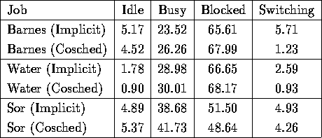
For message latency of 50 s, the spin-wait phase (2  context switch
time) is more than the message latency. Here, the simulated underlying
architecture is a set of tightly coupled processors.
Hence, it is expected that the
processes rarely spin wait (only in the case of lock requests when the
lock is currently being held by another process). As a consequence, the
the implicit scheduling case degenerates to pure local priority scheduling,
with each process occupying the CPU for the entire time slice. In this
situation, co-scheduling as expected, performs better than implicit
scheduling. This can be noticed by observing that the busy time to
idle time ratio is more in co-scheduling than in implicit scheduling.
context switch
time) is more than the message latency. Here, the simulated underlying
architecture is a set of tightly coupled processors.
Hence, it is expected that the
processes rarely spin wait (only in the case of lock requests when the
lock is currently being held by another process). As a consequence, the
the implicit scheduling case degenerates to pure local priority scheduling,
with each process occupying the CPU for the entire time slice. In this
situation, co-scheduling as expected, performs better than implicit
scheduling. This can be noticed by observing that the busy time to
idle time ratio is more in co-scheduling than in implicit scheduling.
Message latency 300 s, Barnes+Water+Sor (3 jobs) % times
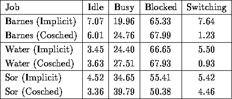
When the message latency is increased to 300 s, the spin-wait phase
for Sor (1600 s) is still greater than
the message latency but not so for Barnes (400 s) and Water
(200 s). In this case,
Sor still favors co-scheduling, whereas in Water, the advantage
of co-scheduling has dwindled. This is because, in Water, processes
are spin-waiting less in implicit scheduling than in co-scheduling.
Barnes, however, has not shown much appreciable change from the
previous case. In fact, it is worse off than the last case (message
latency 50 s), which could possibly be explained by noting that the
Barnes spends a lot of time context switching. In fact, Barnes spends
a lot of time spin-waiting, and is context switched out a little
before the message returns, which is more wasteful.
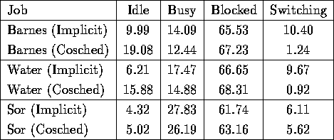
The trend for increasing the message latencies is clear from the
following two cases with even larger latencies.
Message latency 3000 s, Barnes+Water+Sor (3 jobs) % times
Message latency 10000 s, Barnes+Water+Sor (3 jobs) % times
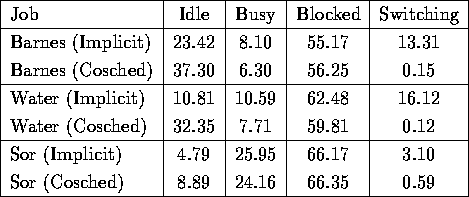
In the above two cases, it is clear that implicit scheduling is a better option than co-scheduling. In both these cases, the spin-wait phase for processes are much smaller than the round trip time of messages. As a consequence, CPUs can be kept more busy if processes context switch out, instead of spin-waiting for message responses.
Although the process spin-wait times have decreased sharply, note that
the time spent context switching has gone up correspondingly in
implicit scheduling. This is expected because in implicit scheduling
the processes context switch in and out more often than in co-scheduling
for larger message latencies. For message latencies of 10000 s,
which is about the delay experienced by packets travelling between
hosts located at two opposite coasts of US, the performance heavily
favors implicit scheduling.
The next table illustrates that with local priority scheduling, as the number of jobs increase, the performance improves. This can be seen by observing that the idle time for each job decreases when there are more jobs. We present the actual times rather than percentages to illustrate the point.
Comparing the implicit scheduling case for three and five jobs, one finds that a process spin-waits for lesser amount of when the number of jobs is higher. This is however, not noticeable in Sor, which is computation intensive.
Message latency 300 s, Time (in secs)
3 jobs - (Barnes+Water+Sor)
5 jobs - (Barnes+Water+Sor+Barnes+Water)
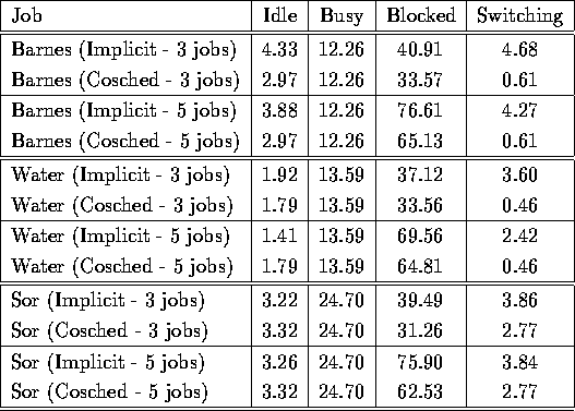
The expectation for this result can be explained by observing the sharper difference in the next table with a larger message latency.
Message latency 3000 s, Time (in secs)
3 jobs - (Barnes+Water+Sor)
5 jobs - (Barnes+Water+Sor+Barnes+Water)
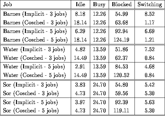
With the message latency kept as 3000 s, as more jobs are
run together, the spin-waiting time of the communication intensive
processes have decreased. The same has not happened for the
computation intensive Sor.
Since when more jobs are running, there are better options for the priority scheduler to select the job that uses the least amount of CPU in its time slice, the jobs that waited longer are re-scheduled.
Since the job waited longer, it is expected that its message would
have returned by the time is gets scheduled. This is not so noticeable
when the message latency was lower (300 s), since messages came
back quicker than the time the job gets re-scheduled. The priority
of processes of Sor are usually low, and hence the difference is
not noticeable for Sor between three and five jobs.
Finally, to compare the advantage of using a priority local scheduler
rather than a pure round-robin scheduler for implicit scheduling, we
also implemented a round-robin local scheduler. The results are
presented in the following table.
Message latency 400 s, Barnes+Water+Sor (3 jobs), Time (in secs)
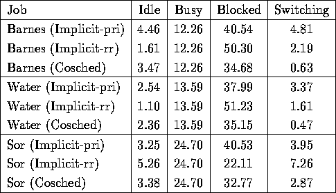
We notice that the blocked time for Sor is more in priority scheduling than in round-robin. This is because, Sor being computation intensive is always given a lower priority than the more communication intensive jobs, Barnes and Water. Also, for the same reason, Barnes and Water are blocked for a larger period in round-robin than in a priority based local scheduler. This, similarly, explains the reverse trend in the idle times. A communication intensive process is scheduled in tn its usual turn in a round-robin, which is later than in the case of priority scheduler, and hence blocks the process long enough to allow the message to return before it is scheduled again. Hence, its idle time decreases.
Analyzing the results, we feel that implicit scheduling is a
better choice as the message latencies between processors increase.
It is definitely competitive with co-scheduling in most of the above
choice of message latencies and clearly better as the latencies get
larger. Also, parameter for the spin-waiting phase should be so
chosen so that the spin-waiting phase is not kept just less
the message round-trip time (as illustrated by comparing the
performance of Barnes for latencies of 50 s and 300 s).