The power of neural networks lies in their ability to generalize to unseen data, yet the underlying reasons for this phenomenon remain elusive. Numerous rigorous attempts have been made to explain generalization, but available bounds are still quite loose, and analysis does not always lead to true understanding. The goal of this work is to make generalization more intuitive. Using visualization methods, we discuss the mystery of generalization, the geometry of loss landscapes, and how the curse (or, rather, the blessing) of dimensionality causes optimizers to settle into minima that generalize well.
The full paper can be found on arxiv:
Ronny Huang has written a blog post about this article that includes very informative animations of the decision boundaries of neural nets. You can find his blog post here.
Why is generalization a mystery?
The generalization ability of neural networks is seemingly at odds with their expressiveness. Neural network training algorithms work by minimizing a loss function that measures model performance using only training data. Because of their flexibility, it is possible to find parameter configurations for neural networks that perfectly fit the training data while making mostly incorrect predictions on test data. Miraculously, commonly used optimizers reliably avoid such “bad” minima of the loss function, and succeed at finding “good” minima that generalize well.

Dancing through a minefield of bad minima: we train a neural net classifier and plot the iterates of SGD after each tenth epoch (red dots). We also plot locations of nearby "bad" minima with poor generalization (blue dots). We visualize these using t-SNE embedding with perplexity 30. All blue dots achieve near perfect train accuracy, but with test accuracy below 53% (random chance is 50%). The final iterate of SGD (black star) also achieves perfect train accuracy, but with 98.5% test accuracy. Miraculously, SGD always finds its way through a landscape full of bad minima, and lands at a minimizer with excellent generalization.
Why are flat minima good?
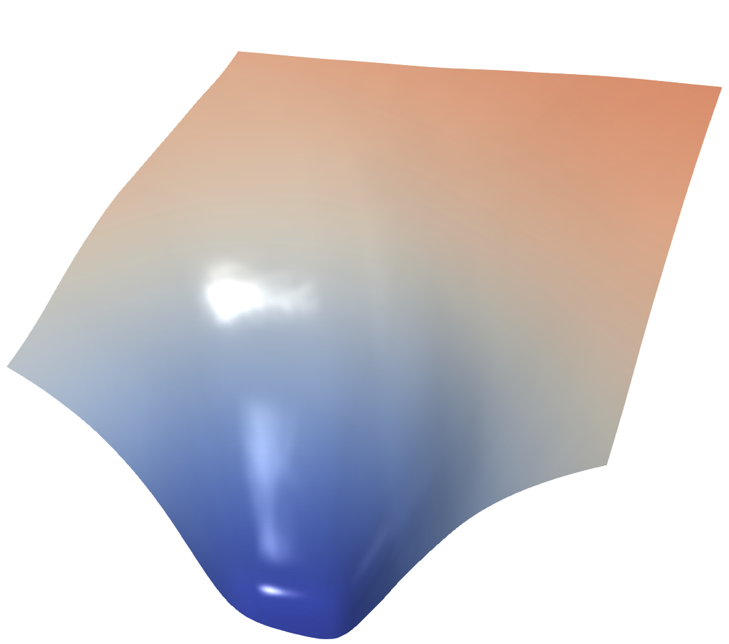
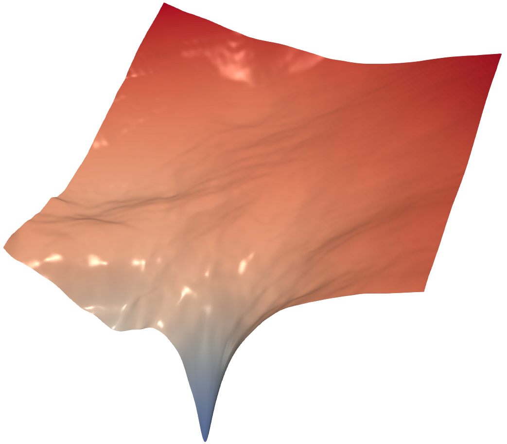
Instead of the classical wide margin regularization of linear classifiers, neural nets rely on implicit regulation that promotes the closely related notion of “flatness” of loss function minima. Flatness is a measure of how sensitive network performance is to perturbations in parameters. Consider a parameter vector that minimizes the loss (i.e., it correctly classifies most if not all training data). If small perturbations to this parameter vector cause a lot of data misclassification, the minimizer is sharp; a small movement away from the optimal parameters causes a large increase in the loss function. In contrast, flat minima have training accuracy that remains nearly constant under small parameter perturbations.
The stability of flat minima to parameter perturbations can be seen as a wide margin condition. When we add random perturbations to network parameters, it causes the class boundaries to wiggle around in space. If the minimizer is flat, then training data lies a safe distance from the class boundary, and perturbing the class boundaries does not change the classification of nearby data points. In contrast, sharp minima have class boundaries that pass close to training data, putting those nearby points at risk of misclassification when the boundaries are perturbed.


Decision boundaries of two networks with different parameters. The network on the left generalizes well. The network on the right generalizes poorly (perfect train accuracy, bad test accuracy). The flatness and large volume of the good minimizer make it likely to be found by SGD, while the sharpness and tiny volume of the bad minimizer make it unlikely to be found. Red and blue dots correspond to the training data.
The volume disparity between flat and sharp minima promotes generalization
The bias of stochastic optimizers towards good minima can be explained by the volume disparity between the attraction basins for good and bad minima. Flat minima that generalize well have wide basins of attraction that occupy a large volume of parameter space. In contrast, sharp minima have narrows basins of attraction that occupy a comparatively small volume of parameter space. As a result, a random search algorithm is more likely to land in the attraction basin for a good minimizer than a bad one.
The volume disparity between good and bad minima is catastrophically magnified by the curse (or, rather, the blessing?) of dimensionality. The differences in width between good and bad basins of attraction does not appear too dramatic in 2D visualizations. However, the probability of colliding with a region during a random search does not scale with its width, but rather its volume. Neural net parameters live in very high-dimensional spaces where small differences in sharpness between minima translate to exponentially large disparities in the volume of their surrounding basins.
To visualize this volume disparity, we find a range of minima for the loss function of a classifier on the SVHN dataset. We define “basins” around each minima to be the nearby points with loss below 0.1. Using a numerical integrator, we compute the volume of each basin, and plot these volumes against the generalization gap of each minimizer. For the SVHN data, we find that bad minima are over 10,000 orders of magnitude smaller than good minima, making them nearly impossible to find by mistake.
