13 Handling Control Hazards
Dr A. P. Shanthi
The objectives of this module are to discuss how to handle control hazards, to differentiate between static and dynamic branch prediction and to study the concept of delayed branching.
A branch in a sequence of instructions causes a problem. An instruction must be fetched at every clock cycle to sustain the pipeline. However, until the branch is resolved, we will not know where to fetch the next instruction from and this causes a problem. This delay in determining the proper instruction to fetch is called a control hazard or branch hazard, in contrast to the data hazards we examined in the previous modules. Control hazards are caused by control dependences. An instruction that is control dependent on a branch cannot be moved in front of the branch, so that the branch no longer controls it and an instruction that is not control dependent on a branch cannot be moved after the branch so that the branch controls it. This will give rise to control hazards.
The two major issues related to control dependences are exception behavior and handling and preservation of data flow. Preserving exception behavior requires that any changes in instruction execution order must not change how exceptions are raised in program. That is, no new exceptions should be generated.
| • Example: | |
| ADD | R2,R3,R4 |
| BEQZ | R2,L1 |
| LD | R1,0(R2) |
| L1: |
What will happen with moving LD before BEQZ? This may lead to memory protection violation. The branch instruction is a guarding branch that checks for an address zero and jumps to L1. If this is moved ahead, then an additional exception will be raised. Data flow is the actual flow of data values among instructions that produce results and those that consume them. Branches make flow dynamic and determine which instruction is the supplier of data
• Example:
| DADDU | R1,R2,R3 |
| BEQZR4,L |
| DSUBU | R1,R5,R6 |
| L:… | |
| OR | R7,R1,R8 |
The instruction OR depends on DADDU or DSUBU? We must ensure that we preserve data flow on execution.
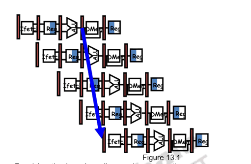
The general rule to reduce branch penalties is to resolve branches as early as possible. In the MIPS pipeline, the comparison of registers and target address calculation is normally done at the execution stage. This gives rise to three clock cycles penalty. This is indicated in Figure 13.1. If we do a more aggressive implementation by adding hardware to resolve the branch in the ID stage, the penalty can be reduced.
Resolving the branch earlier requires two actions to occur – computing the branch target address and evaluating the branch decision early. The easy part of this change is to move up the branch address calculation. We already have the PC value and the immediate field in the IF/ID pipeline register, so we just move the branch adder from the EX stage to the ID stage; of course, the branch target address calculation will be performed for all instructions, but only used when needed. The harder part is the branch decision itself. For branch equal, we would compare the two registers read during the ID stage to see if they are equal. Equality can be tested by first exclusive ORing their respective bits and then ORing all the results. Moving the branch test to the ID stage also implies additional forwarding and hazard detection hardware, since a branch dependent on a result still in the pipeline must still work properly with this optimization. For example, to implement branch-on-equal (and its inverse), we will need to forward results to the equality test logic that operates during ID. There are two complicating factors:
- During ID, we must decode the instruction, decide whether a bypass to the equality unit is needed, and complete the equality comparison so that if the instruction is a branch, we can set the PC to the branch target address. Forwarding for the operands of branches was formerly handled by the ALU forwarding logic, but the introduction of the equality test unit in ID will require new forwarding logic. Note that the bypassed source operands of a branch can come from either the ALU/MEM or MEM/WB pipeline latches.
- Because the values in a branch comparison are needed during ID but may be produced later in time, it is possible that a data hazard can occur and a stall will be needed. For example, if an ALU instruction immediately preceding a branch produces one of the operands for the comparison in the branch, a stall will be required, since the EX stage for the ALU instruction will occur after the ID cycle of the branch.
Despite these difficulties, moving the branch execution to the ID stage is an improvement since it reduces the penalty of a branch to only one instruction if the branch is taken, namely, the one currently being fetched.
There are basically two ways of handling control hazards:
1. Stall until the branch outcome is known or perform the fetch again
2. Predict the behavior of branches
a. Static prediction by the compiler
b. Dynamic prediction by the hardware
The first option of stalling the pipeline till the branch is resolved, or fetching again from the resolved address leads to too much of penalty. Branches are very frequent and not handling them effectively brings down the performance. We are also violating the principle of “Make common cases fast”.
The second option is predicting about the behavior of branches. Branch Prediction is the ability to make an educated guess about which way a branch will go – will the branch be taken or not. First of all, we shall discuss about static prediction done by the compiler. This is based on typical branch behavior. For example, for loop and if-statement branches, we can predict that backward branches will be taken and forward branches will not be taken. So, there are primarily three methods adopted. They are:
– Predict not taken approach
• Assume that the branch is not taken, i.e. the condition will not evaluate to be true
– Predict taken approach
• Assume that the branch is taken, i.e. the condition will evaluate to be true
– Delayed branching
• A more effective solution
In the predict not taken approach, treat every branch as “not taken”. Remember that the registers are read during ID, and we also perform an equality test to decide whether to branch or not. We simply load in the next instruction (PC+4) and continue. The complexity arises when the branch evaluates to be true and we end up needing to actually take the branch. In such a case, the pipeline is cleared of any code loaded from the “not-taken” path, and the execution continues.
In the predict-taken approach, we assume that the branch is always taken. This method will work for processors that have the target address computed in time for the IF stage of the next instruction so there is no delay, and the condition alone may not be evaluated. This will not work for the MIPS architecture with a 5-stage pipeline. Here, the branch target is computed during the ID cycle or later and the condition is also evaluated in the same clock cycle.
The third approach is the delayed branching approach. In this case, an instruction that is useful and not dependent on whether the branch is taken or not is inserted into the pipeline. It is the job of the compiler to determine the delayed branch instructions. The slots filled up by instructions which may or may not get executed, depending on the outcome of the branch, are called the branch delay slots. The compiler has to fill these slots with useful/independent instructions. It is easier for the compiler if there are less number of delay slots.
There are three different ways of introducing instructions in the delay slots:
• Before branch instruction
• From the target address: only valuable when branch taken
• From fall through: only valuable when branch is not taken
• Cancelling branches allow more slots to be filled
Figure 13.2 shows the three different ways of filling in instructions in the branch delay slots.
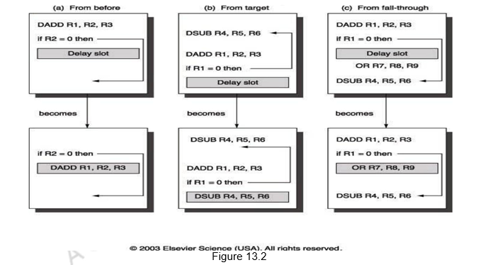
When the first choice is taken, the branch must not depend on the rescheduled instructions and there will always be performance improvement, irrespective of which way the branch goes. When instructions are picked from the target path, the compiler predicts that the branch is going to take. It must be alright to execute rescheduled instructions even if the branch is not taken. That is, the work may be wasted, but the program will still execute correctly. This may need duplication of instructions. There will be improvement in performance only when the branch is taken. When the branch is not taken, the extra instructions may increase the code size. When instructions are picked from the fall through path, the compiler predicts that the branch is not going to take. It must be alright to execute rescheduled instructions even if the branch is taken. This may lead to improvement in performance only if the branch is not taken. The extra instructions added as compensatory code may be an overhead.
The limitations on delayed-branch scheduling arise from (1) the restrictions on the instructions that are scheduled into the delay slots and (2) our ability to predict at compile time whether a branch is likely to be taken or not. If the compiler is not able to find useful instructions, it may fill up the slots with nops, which is not a good option.
To improve the ability of the compiler to fill branch delay slots, most processors with conditional branches have introduced a cancelling or nullifying branch. In a cancelling branch, the instruction includes the direction that the branch was predicted. When the branch behaves as predicted, the instruction in the branch delay slot is simply executed as it would normally be with a delayed branch. When the branch is incorrectly predicted, the instruction in the branch delay slot is simply turned into a no-op. Examples of such branches are Cancel-if-taken or Cancel-if-not-taken branches. In such cases, the compiler need not be too conservative in filling the branch delay slots, because it knows that the hardware will cancel the instruction if the branch behavior goes against the prediction.
The pipeline speedup is given by
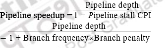
Let us look at an example to calculate the speedup, given the following:
14% Conditional & Unconditional, 65% Taken; 52% Delay slots not usefully filled. The details for the various schemes are provided in the table below.
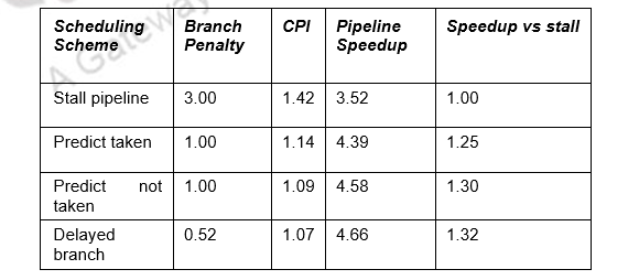
• Stall: 1+.14(branches)*3(cycle stall)
• Taken: 1+.14(branches)*(.65(taken)*1(delay to find address)+.35(not taken)*1(penalty))
• Not taken: 1+.14*(.65(taken)*1+[.35(not taken)*0])
• Delayed: 1+.14*(.52(not usefully filled)*1)
Other example problems:
Given an application where 20% of the instructions executed are conditional branches and 59% of those are taken. For the MIPS 5-stage pipeline, what speedup will be achieved using a scheme where all branches are predicted as taken over a scheme with no branch prediction (i.e. branches will always incur a 1 cycle penalty)? Ignore all other stalls.
• CPI with no branch prediction
= 0.8 x 1 + 0.2 x 2 = 1.2
• CPI with branch prediction
= 0.8 x 1 + 0.2 x 0.59 x 1 + 0.2 x 0.41 x 2 = 1.082
• Speed up = 1.2 / 1.082 = 1.109
We want to compare the performance of two machines. Which machine is faster?
• Machine A: Dual ported memory – so there are no memory stalls
• Machine B: Single ported memory, but its pipelined implementation has a 1.05 times faster clock rate
Assume:
• Ideal CPI = 1 for both
• Loads are 40% of instructions executed SpeedUpA
= Pipeline Depth/(1 + 0) x (clockunpipe/clockpipe)
= Pipeline Depth
SpeedUpB
- = Pipeline Depth/(1 + 0.4 x 1) x (clockunpipe/(clockunpipe / 1.05)
- = (Pipeline Depth/1.4) x 1.05
- = 75 x Pipeline Depth
SpeedUpA / SpeedUpB
- = Pipeline Depth / (0.75 x Pipeline Depth) = 1.33 Machine A is 1.33 times faster
To summarize, we have discussed about control hazards that arise due to control dependences caused by branches. Branches are very frequent and so have to be handled properly. There are different ways of handling branch hazards. The pipeline can be stalled, but that is not an effective way to handle branches. We discussed the predict taken, predict not taken and delayed branching techniques to handle branch hazards. All these are static techniques. We will discuss further on branch hazards in the next module.
Web Links / Supporting Materials
- Computer Organization and Design – The Hardware / Software Interface, David A. Patterson and John L. Hennessy, 4th.Edition, Morgan Kaufmann, Elsevier, 2009.
- Computer Organization, Carl Hamacher, Zvonko Vranesic and Safwat Zaky, 5th.Edition, McGraw- Hill Higher Education, 2011.